Smart Beta 2.0 - EDHEC-Risk

More documents

Recommendations

Info

2. Controlling the Risks of Smart Beta Investing: The Smart Beta 2.0 Approach The second generation of smart beta clearly poses the problem of measuring and controlling the risks of these new forms of indices. Even though the majority of smart beta indices have a strong probability of outperforming cap-weighted indices over the long term because of the high level of concentration of the latter, it should be noted that through their exposure to sources of risk that are different from those of cap-weighted indices, these new benchmarks can sometimes significantly underperform market indices for a considerable length of time. The exhibit below shows the magnitude and duration of the worst underperformance for a range of smart beta indices. Please refer to the Appendix for a brief description of the smart beta strategies included in this table. The results show that smart beta strategies can encounter severe relative drawdowns relative to the cap-weighted reference index which are at least in the order of 10%. Moreover, as the time under water statistics suggest, underperformance can last for extended time periods. 2.1 Choosing and Controlling Exposure to Systematic Risk Factors Paying attention to the systematic risks of smart beta is today not only a genuine opportunity to create added value, but is also a condition for its durability. While smart beta can play an important role in institutional investors’ allocations, we think that this can only be at the price of implementing a genuine risk management process. It would seem fairly contradictory for investors to accept the idea that what drives their global asset allocation is more the integration of the risks of asset classes or categories rather than the names of the latter (as evidenced by increasing interest in modern approaches which look at risks rather than asset categories when defining an allocation, as for example in the risk parity and more generally in risk allocation approaches) and that they forget to look into the risks of the benchmarks used to invest in these asset categories. The first approach to take into account the systematic risks of investing in smart beta Exhibit 8: Relative risk of various alternative beta strategies – The table summarises the maximum relative drawdown numbers for selected commercial smart beta indices and 10 Scientific Beta USA flagship Indices with respect to the S&P 500 Index. Maximum relative drawdown is the maximum drawdown of the long-short index whose return is given by the fractional change in the ratio of strategy index to the benchmark index. Daily total return data for the period 23 December 2002 to 31 December 2012 has been used for the analysis as this is the earliest date since data for all indices are available. Returns data has been downloaded from Datastream and from www.scientificbeta.com. Indices from Traditional Index Providers Scientific Beta USA Flagship Indices Maximum Relative Drawdown Time Under Water (business days) FTSE RAFI U.S. 1000 Index 12.71% 439 FTSE EDHEC Risk Efficient U.S. Index 8.72% 46 MSCI USA Minimum Volatility Index 12.82% 371 S&P 500 Equal Weight Index 13.72% 453 High Liquidity Max Decorrelation 14.27% 104 High Liquidity Max Deconcentration 15.53% 110 High Liquidity Efficient Max Sharpe 10.14% 103 High Liquidity Efficient Min Volatility 6.17% 507 Low Volatility Max Deconcentration 7.75% 222 Value Max Deconcentration 15.30% 44 Growth Max Deconcentration 26.42% 1299 High Dividend Yield Max Deconcentration 16.65% 112 16
2. Controlling the Risks of Smart Beta Investing: The Smart Beta 2.0 Approach that we feel is very compatible with the idea that an index must remain a simple construction is the disentangling of the two ingredients that form the basis of any smart beta index construction scheme: the stock selection and weighting phases. A very clear separation of the selection and weighting phases enables investors to choose the risks to which they do or do not wish to be exposed. This choice of risk is expressed firstly by a very specific and controlled definition of the investment universe. An investor wishing to avail of a better diversified benchmark than a capweighted index but disinclined to take on liquidity risk can decide to apply this scheme solely to a very liquid selection of stocks. In the same way, an investor who does not want the diversification of his benchmark to lead him to favour stocks with a value bias can absolutely decide that the diversification method chosen will only be applied to growth, or at least not strictly value, stocks, etc. In an article published recently in the Journal of Portfolio Management (Amenc, Goltz and Lodh 2012) we have been able to show that the distinction between the selection and weighting phases (which can be made for most smart beta construction methods) could add value both in terms of performance and in controlling the investment risks. Exhibits 9 and 10 reproduce some of the results in the article. 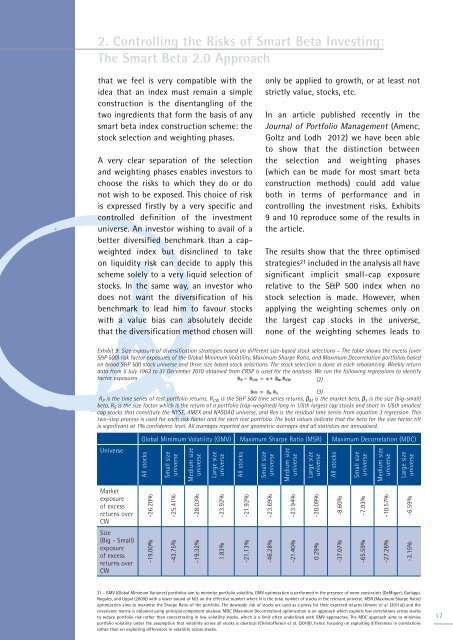The results show that the three optimised strategies 21 included in the analysis all have significant implicit small-cap exposure relative to the S&P 500 index when no stock selection is made. However, when applying the weighting schemes only on the largest cap stocks in the universe, none of the weighting schemes leads to Exhibit 9: Size exposure of diversification strategies based on different size-based stock selections – The table shows the excess (over S&P 500) risk factor exposures of the Global Minimum Volatility, Maximum Sharpe Ratio, and Maximum Decorrelation portfolios based on broad S&P 500 stock universe and three size based stock selections. The stock selection is done at each rebalancing. Weekly return data from 5 July 1963 to 31 December 2010 obtained from CRSP is used for the analysis. We run the following regressions to identify factor exposures (2) (3) R P is the time series of test portfolio returns, R CW is the S&P 500 time series returns, β M is the market beta, β S is the size (big-small) beta, R S is the size factor which is the return of a portfolio (cap-weighted) long in 1/5th largest cap stocks and short in 1/5th smallest cap stocks that constitute the NYSE, AMEX and NASDAQ universe, and Res is the residual time series from equation 3 regression. This two-step process is used for each risk factor and for each test portfolio. The bold values indicate that the beta for the size factor tilt is significant at 1% confidence level. All averages reported are geometric averages and all statistics are annualised. Universe Global Minimum Volatility (GMV) Maximum Sharpe Ratio (MSR) Maximum Decorrelation (MDC) All stocks Small size universe Medium size universe Large size universe All stocks Small size universe Medium size universe Large size universe All stocks Small size universe Medium size universe Large size universe Market exposure of excess returns over CW -26.20% -25.41% -28.03% -23.92% -21.92% -23.69% -23.94% -20.09% -8.60% -7.93% -10.57% -6.59% Size (Big - Small) exposure of excess returns over CW -19.00% -43.75% -19.32% 1.83% -21.13% -46.28% -21.40% 0.29% -37.07% -65.59% -27.26% -3.15% 21 - GMV (Global Minimum Variance) portfolios aim to minimise portfolio volatility. GMV optimization is performed in the presence of norm constraints (DeMiguel, Garlappi, Nogales, and Uppal (2009)) with a lower bound of N/3 on the effective number where N is the total number of stocks in the relevant universe. MSR (Maximum Sharpe Ratio) optimization aims to maximise the Sharpe Ratio of the portfolio. The downside risk of stocks are used as a proxy for their expected returns (Amenc et al. (2011a)) and the covariance matrix is obtained using principal component analysis. MDC (Maximum Decorrelation) optimization is an approach which exploits low correlations across stocks to reduce portfolio risk rather than concentrating in low volatility stocks, which is a limit often underlined with GMV approaches. The MDC approach aims to minimise portfolio volatility under the assumption that volatility across all stocks is identical (Christoffersen et al. (2010)), hence focusing on exploiting differences in correlations rather than on exploiting differences in volatility across stocks. 17
Page 1 and 2: Smart Beta 2.0 March 2013 Noël Ame
Page 3 and 4: About the Authors Noël Amenc is pr
Page 5 and 6: Introduction: Taking the Risks of S
Page 7 and 8: 1. The Risks of Smart Beta Strategi
Page 15: 1. The Risks of Smart Beta Strategi
Page 19 and 20: 2. Controlling the Risks of Smart B
Page 25 and 26: Conclusion: Smart Beta 2.0 — New
Page 27 and 28: References • Amenc, N. and F. Duc
Page 29 and 30: References • Jagannathan, R., and
Page 31 and 32: EDHEC-Risk Institute Position Paper
Page 33 and 34: EDHEC-Risk Institute Position Paper
Page 36: Founded in 1906, EDHEC Business Sch

Smart Beta 2.0 - EDHEC-Risk

You also want an ePaper? Increase the reach of your titles

Delete template?

Save as template?