Estimating Distributions of Counterfactuals with an Application ... - UCL

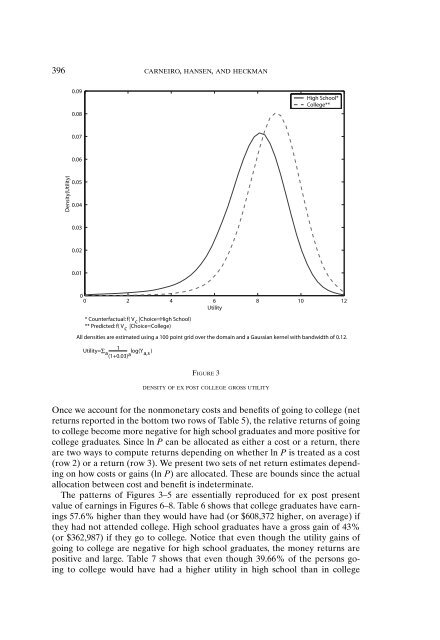
396 CARNEIRO, HANSEN, AND HECKMAN
0.09
0.08
High School*
College**
0.07
0.06
Density(Utility)
0.05
0.04
0.03
0.02
0.01
0
0 2 4 6 8 10 12
Utility
* Counterfactual: f( V c |Choice=High School)
** Predicted: f( V c |Choice=College)
All densities are estimated using a 100 point grid over the domain and a Gaussian kernel with bandwidth of 0.12.
Utility=
1
Σ a(1+0.03) a log(Y a,s )
FIGURE 3
DENSITY OF EX POST COLLEGE GROSS UTILITY
Once we account for the nonmonetary costs and benefits of going to college (net
returns reported in the bottom two rows of Table 5), the relative returns of going
to college become more negative for high school graduates and more positive for
college graduates. Since ln P can be allocated as either a cost or a return, there
are two ways to compute returns depending on whether ln P is treated as a cost
(row 2) or a return (row 3). We present two sets of net return estimates depending
on how costs or gains (ln P) are allocated. These are bounds since the actual
allocation between cost and benefit is indeterminate.
The patterns of Figures 3–5 are essentially reproduced for ex post present
value of earnings in Figures 6–8. Table 6 shows that college graduates have earnings
57.6% higher than they would have had (or $608,372 higher, on average) if
they had not attended college. High school graduates have a gross gain of 43%
(or $362,987) if they go to college. Notice that even though the utility gains of
going to college are negative for high school graduates, the money returns are
positive and large. Table 7 shows that even though 39.66% of the persons going
to college would have had a higher utility in high school than in college