Estimating Distributions of Counterfactuals with an Application ... - UCL

More documents

Recommendations

Info

410 CARNEIRO, HANSEN, AND HECKMAN than 16 years in school. We exclude the oversample of poor whites. Experience is Mincer experience (age-12 if high-school graduate, age-16 for college graduate). The variables that we include in the outcome and choice equations are number of siblings, parental years of schooling, AFQT, year of birth dummies, average tuition of the colleges in the county the individual lives in at 17 (we simulate the policy change by decreasing this variable by $1000 for each individual), distance to the nearest college at 17, average local blue collar wage in state of residence at 17 (or in 1979, for individuals entering the sample at ages older than 17) and local unemployment rate in the county of residence in 1979. For the construction of the tuition variable see Cameron and Heckman (2001). Distance to college is constructed by matching college location data in HEGIS (Higher Education General Information Survey) with county of residence in NLSY. State average blue collar wages are constructed by using data from the BLS. For a description of the NLSY sample see BLS (2001). In 1980, NLSY respondents were administered a battery of 10 achievement tests referred to as the Armed Forces Vocational Aptitude Battery (ASVAB; see Cawley et al., 1997, for a complete description). The math and verbal components of the ASVAB can be aggregated into the Armed Forces Qualification Test (AFQT) scores. 40 Many studies have used the overall AFQT score as a control variable, arguing that this is a measure of scholastic ability. We argue that AFQT is an imperfect proxy for scholastic ability and use the factor structure to capture this. We also avoid a potential aggregation bias by using each of the components of the ASVAB as a separate measure. For our analysis, we use the random sample of the NLSY and restrict the sample to 1161 white males for whom we have information on schooling, several parental background variables, test scores, and behavior. Distance to nearest college at each date is constructed in the following way: Take the county of residence of each individual and all other counties within the same state. The distance between two counties is defined as the distance between the center of each county. If there exists a college (2-year or 4-year) in the county of residence where a person lives then the distance to the nearest college (2-year or 4-year) variable takes the value of zero. Otherwise, we compute distance (in miles) to the nearest county with a college. Then we construct the distance to the nearest college at 17 by using the county of residence at 17. However, for people who were older than 17 in 1979 we use the county of residence in 1979 for the construction of this variable. Tuition at age 17 is average tuition in colleges in the county of residence at 17. If there is no college in the county then average tuition in the state is taken instead. For details on the construction of this variable see Cameron and Heckman (2001). Local labor market variables for the county of residence are computed using information in the 5% sample of the 1980 Census. For each county group in the census we compute the local unemployment rate and average wage for high school 40 Implemented in 1950, the AFQT score is used by the army to screen draftees.
EFFECTS OF UNCERTAINTY ON COLLEGE CHOICE 411 dropouts, high school graduates, individuals with some college, and four-year college graduates. We do not have this variable for years other than 1980 so, for each county, we assume that it is a good proxy for local labor market conditions in all the other years where NLSY respondents are assumed to be making the schooling decisions we consider in this article. We also use the variable log annual labor earnings. We extract this variable from the NLSY79 reported annual earnings from wages and salary. Earnings (in thousands of dollars) are discounted to 1993 using the Consumer Price Index reported by the Bureau of Labor Statistics. Missing values for this variable may occur here for two reasons: first, because respondents do not report earnings from wages/salary, and second, because the NLSY becomes biannual after 1994 and this prevents us from observing respondents when they reach certain ages. For example, because the NLSY79 was not conducted in 1995, we do not observe individuals born in 1964 when they are 31-year-olds. In this case we input missing values. To predict missing log earnings between ages 19 and 35 and extrapolate from age 36 to 65 years we pool NLSY and PSID data. From the latter, we use the sample of white males that are household heads and that are either high school or college graduates according to the definition given above. This produces a sample of 3043 individuals from the PSID. To get annual earnings, we multiply the reported CPIadjusted (1993 = 100) hourly wage rate by the annual hours worked and divide the outcome by 1000. Then we take logs to have an NLSY-comparable variable. Similarly to NLSY, we generate the Mincerian experience according to the rule given above. We also generate dummy variables for cohorts. The first (omitted) cohort, consists of individuals born between 1896 and 1905, the second consists of individuals born between 1906 and 1915, and so on up to the last cohort, which is made up of PSID respondents born between 1976 and 1985. We pool NLSY and PSID by merging the NLSY respondents in the PSID cohort born between 1956 and 1965. 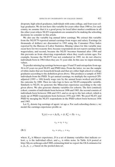Let Y ia denote log earnings of agent i at age a. For each schooling choice s, we model the earnings-experience profile as Y ia (s) = α + β 0 X ia + β 1 X 2 ia + Dγ + ε ia ε ia = η i + v ia (B.1) v ia = ρv ia−1 + κ ia where X ia is Mincer experience, D is a set of dummy variables that indicate cohort, η i is the individual effect, and κ ia is white noise. In Table A14 posted at http://lily.src.uchicago.edu/CHH estimating.html we report the OLS estimates for α, β 0 ,β 1 ,γ,ρ based on the pooled data set.
Page 1 and 2: INTERNATIONAL ECONOMIC REVIEW May 2
Page 3 and 4: EFFECTS OF UNCERTAINTY ON COLLEGE C
Page 49: EFFECTS OF UNCERTAINTY ON COLLEGE C

Estimating Distributions of Counterfactuals with an Application ... - UCL

You also want an ePaper? Increase the reach of your titles

Delete template?

Save as template?