Estimating Distributions of Counterfactuals with an Application ... - UCL

More documents

Recommendations

Info

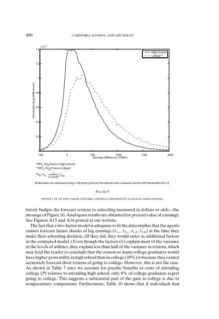
400 CARNEIRO, HANSEN, AND HECKMAN 1.4 x10-3 High School* College** 1.2 1 Density(Earnings Differences) 0.8 0.6 0.4 0.2 0 -500 0 500 1000 1500 2000 Earnings Differences (1000's) *f(PV c -PV h |Choice=High School) **f(PV c -PV h |Choice=College) PV 1 h = Σ a (1+0.03) a Y h,a All densities are estimated using a 100 point grid over the domain and a Gaussian kernel with bandwidth of 0.12. FIGURE 6 DENSITY OF EX POST GROSS LIFETIME EARNINGS DIFFERENCES (COLLEGE–HIGH SCHOOL) barely budges the forecast returns to schooling measured in dollars or utils—the message of Figure 10. Analogous results are obtained for present value of earnings. See Figures A15 and A16 posted at our website. The fact that a two-factor model is adequate to fit the data implies that the agents cannot forecast future shocks of log earnings (¯ε 1,c , ¯ε 2,c , ¯ε 1,h , ¯ε 2,h ) at the time they make their schooling decision. (If they did, they would enter as additional factors in the estimated model.) Even though the factors (θ) explain most of the variance in the levels of utilities, they explain less than half of the variance in returns, which may lead the reader to conclude that the reason so many college graduates would have higher gross utility in high school than in college (39%) is because they cannot accurately forecast their returns of going to college. However, this is not the case. As shown in Table 7 once we account for psychic benefits or costs of attending college (P) relative to attending high school, only 8% of college graduates regret going to college. This suggests a substantial part of the gain to college is due to nonpecuniary components. Furthermore, Table 10 shows that if individuals had
EFFECTS OF UNCERTAINTY ON COLLEGE CHOICE 401 0.9 1 High School* College** 0.8 0.7 Density(Returns) 0.6 0.5 0.4 0.3 0.2 0.1 0 -0.5 0 0.5 1 1.5 2 2.5 Returns *f((PV c /PV h )-1|Choice=High School) **f((PV c /PV h )-1|Choice=College) PV 1 h = Σ a (1+0.03) a Y h,a All densities are estimated using a 100 point grid over the domain and a Gaussian kernel with bandwidth of 0.12. FIGURE 7 DENSITY OF EX POST RELATIVE GROSS EARNINGS DIFFERENCES (COLLEGE–HIGH SCHOOL) knowledge of (¯ε 1,c , ¯ε 2,c , ¯ε 1,h , ¯ε 2,h ), keeping their average expected earnings the same, very few of them would change their schooling decision. Uncertainty in gains to schooling is substantial but knowledge of this uncertainty has a very small effect on the choice of schooling because the variance of gains is so much smaller than the variance of psychic costs or benefits, and it is the latter that drives most of the heterogeneity in schooling decisions. In addition, there is uncertainty about the level of both college and high school earnings. See the variances reported for each in Table 9. The uncertainty in the return comes from both sources although the literature emphasizes the uncertainty in college earnings. When conducting this experiment, we make sure that the average expected earnings are the same because a mean preserving reduction in the uncertainty faced by the agents in terms of utility is not the same as a mean preserving change in uncertainty in terms of levels of earnings (see Appendix D). 34 In particular, a change in the variance of (¯ε 1,c , ¯ε 2,c , ¯ε 1,h , ¯ε 2,h ) would not change the expected utility in each schooling level 34 See the numbers posted at the website.
Page 1 and 2: INTERNATIONAL ECONOMIC REVIEW May 2
Page 3 and 4: EFFECTS OF UNCERTAINTY ON COLLEGE C
Page 39: EFFECTS OF UNCERTAINTY ON COLLEGE C

Estimating Distributions of Counterfactuals with an Application ... - UCL

You also want an ePaper? Increase the reach of your titles

Delete template?

Save as template?