Estimating Distributions of Counterfactuals with an Application ... - UCL
Estimating Distributions of Counterfactuals with an Application ... - UCL
Estimating Distributions of Counterfactuals with an Application ... - UCL

You also want an ePaper? Increase the reach of your titles
YUMPU automatically turns print PDFs into web optimized ePapers that Google loves.
398 CARNEIRO, HANSEN, AND HECKMAN<br />
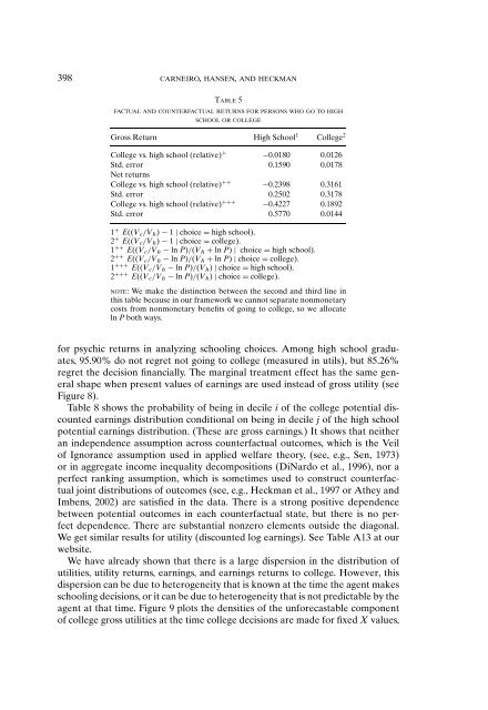
TABLE 5<br />
FACTUAL AND COUNTERFACTUAL RETURNS FOR PERSONS WHO GO TO HIGH<br />
SCHOOL OR COLLEGE<br />
Gross Return High School 1 College 2<br />
College vs. high school (relative) + −0.0180 0.0126<br />
Std. error 0.1590 0.0178<br />
Net returns<br />
College vs. high school (relative) ++ −0.2398 0.3161<br />
Std. error 0.2502 0.3178<br />
College vs. high school (relative) +++ −0.4227 0.1892<br />
Std. error 0.5770 0.0144<br />
1 + E((V c /V h ) − 1 | choice = high school).<br />
2 + E((V c /V h ) − 1 | choice = college).<br />
1 ++ E((V c /V h − ln P)/(V h + ln P) | choice = high school).<br />
2 ++ E((V c /V h − ln P)/(V h + ln P) | choice = college).<br />
1 +++ E((V c /V h − ln P)/(V h ) | choice = high school).<br />
2 +++ E((V c /V h − ln P)/(V h ) | choice = college).<br />
NOTE: We make the distinction between the second <strong>an</strong>d third line in<br />
this table because in our framework we c<strong>an</strong>not separate nonmonetary<br />
costs from nonmonetary benefits <strong>of</strong> going to college, so we allocate<br />
ln P both ways.<br />
for psychic returns in <strong>an</strong>alyzing schooling choices. Among high school graduates,<br />
95.90% do not regret not going to college (measured in utils), but 85.26%<br />
regret the decision fin<strong>an</strong>cially. The marginal treatment effect has the same general<br />
shape when present values <strong>of</strong> earnings are used instead <strong>of</strong> gross utility (see<br />
Figure 8).<br />
Table 8 shows the probability <strong>of</strong> being in decile i <strong>of</strong> the college potential discounted<br />
earnings distribution conditional on being in decile j <strong>of</strong> the high school<br />
potential earnings distribution. (These are gross earnings.) It shows that neither<br />
<strong>an</strong> independence assumption across counterfactual outcomes, which is the Veil<br />
<strong>of</strong> Ignor<strong>an</strong>ce assumption used in applied welfare theory, (see, e.g., Sen, 1973)<br />
or in aggregate income inequality decompositions (DiNardo et al., 1996), nor a<br />
perfect r<strong>an</strong>king assumption, which is sometimes used to construct counterfactual<br />
joint distributions <strong>of</strong> outcomes (see, e.g., Heckm<strong>an</strong> et al., 1997 or Athey <strong>an</strong>d<br />
Imbens, 2002) are satisfied in the data. There is a strong positive dependence<br />
between potential outcomes in each counterfactual state, but there is no perfect<br />
dependence. There are subst<strong>an</strong>tial nonzero elements outside the diagonal.<br />
We get similar results for utility (discounted log earnings). See Table A13 at our<br />
website.<br />
We have already shown that there is a large dispersion in the distribution <strong>of</strong><br />
utilities, utility returns, earnings, <strong>an</strong>d earnings returns to college. However, this<br />
dispersion c<strong>an</strong> be due to heterogeneity that is known at the time the agent makes<br />
schooling decisions, or it c<strong>an</strong> be due to heterogeneity that is not predictable by the<br />
agent at that time. Figure 9 plots the densities <strong>of</strong> the unforecastable component<br />
<strong>of</strong> college gross utilities at the time college decisions are made for fixed X values,