Estimating Distributions of Counterfactuals with an Application ... - UCL

More documents

Recommendations

Info

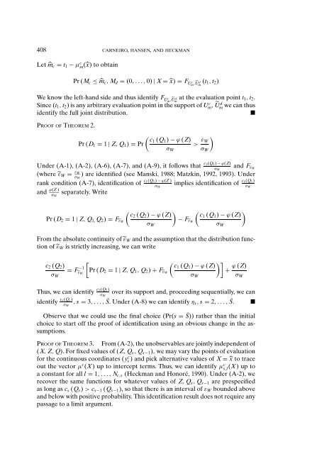
408 CARNEIRO, HANSEN, AND HECKMAN Let ̂m c = t 1 − µ c m (̂x) to obtain Pr (M c ≤ ̂m c , M d = (0,...,0) | X = ̂x) = F U c m ,Ũ d m (t 1, t 2 ) We know the left-hand side and thus identify F U c m ,Ũ at the evaluation point t 1, t m d 2 . Since (t 1 , t 2 ) is any arbitrary evaluation point in the support of Um c , Ũd m we can thus identify the full joint distribution. PROOF OF THEOREM 2. ( c1 (Q 1 ) − ϕ (Z) Pr (D 1 = 1 | Z, Q 1 ) = Pr > ε ) W σ W σ W Under (A-1), (A-2), (A-6), (A-7), and (A-9), it follows that c 1(Q 1 ) − ϕ(Z) σ W and F˜εW (where ˜ε W = ε W σW ) are identified (see Manski, 1988; Matzkin, 1992, 1993). Under rank condition (A-7), identification of c 1(Q 1 ) − ϕ(Z ) σ W implies identification of c 1(Q 1 ) σ W and ϕ(Z ) σ W separately. Write ( ) ( ) c2 (Q 2 ) − ϕ (Z) c1 (Q 1 ) − ϕ (Z) Pr (D 2 = 1 | Z, Q 1, Q 2 ) = F˜εW − F˜εW σ W σ W From the absolute continuity of˜ε W and the assumption that the distribution function of˜ε W is strictly increasing, we can write c 2 (Q 2 ) σ W [ ( )] = F −1 c1 (Q 1 ) − ϕ (Z) ˜ε W Pr (D 2 = 1 | Z, Q 1 , Q 2 ) + F˜εW + ϕ (Z) σ W σ W Thus, we can identify c 2(Q 2) σ W over its support and, proceeding sequentially, we can identify c s(Q s) σ W , s = 3,...,S. Under (A-8) we can identify η s , s = 2,...,S. Observe that we could use the final choice (Pr(s = S)) rather than the initial choice to start off the proof of identification using an obvious change in the assumptions. PROOF OF THEOREM 3. From (A-2), the unobservables are jointly independent of (X, Z, Q). For fixed values of (Z, Q s , Q s−1 ), we may vary the points of evaluation for the continuous coordinates (ys c ) and pick alternative values of X = ̂x to trace out the vector µ c (X) up to intercept terms. Thus, we can identify µ c s,l (X) upto a constant for all l = 1,...,N c,s (Heckman and Honoré, 1990). Under (A-2), we recover the same functions for whatever values of Z, Q s , Q s−1 are prespecified as long as c s (Q s ) > c s−1 (Q s−1 ), so that there is an interval of ε W bounded above and below with positive probability. This identification result does not require any passage to a limit argument.
EFFECTS OF UNCERTAINTY ON COLLEGE CHOICE 409 For values of (Z, Q s , Q s−1 ) such that lim Pr (D Qs → ¯Qs (Z ) s = 1 | Z, Q s , Q s−1 ) = 1 Q s−1 →Q s−1 (Z ) where ¯Q s (Z) is an upper limit and Q s−1 (Z) is a lower limit, and we allow the limits to depend on Z, we essentially integrate out˜ε W and obtain Pr ( M c ≤ m c , ˜µ d m ≤−Ud m , Uc s ≤ yc s − µc (X), Ũ d s ≤−˜µ d s (X)) We know that this probability can be achieved by virtue of the support condition of Assumption (A-10). Then proceeding as in the proof of Theorem 1, we can identify ˜µ d s (X) coordinate by coordinate and we obtain the constants in µ c s,l (X), l = 1,...,N c,s as well as the constants in ˜µ d (X). From the assumption of mean or median zero of the unobservables. In this exercise, we use the full rank condition on X, which is part of Assumption (A-11). With these functions in hand, under the full conditions of Assumption (A-10), we can fix ys c, yc m , ˜µd s , ˜µd m , c s(Q s) − ϕ(Z) σ W , c s−1(Q s−1) − ϕ(Z) σ W at different values to trace out the joint distribution F(Um c , Ũd m , Uc s , Ũd s ,˜ε W). 39 APPENDIX B: DESCRIPTION OF THE DATA We use white males from NLSY79. In the original sample there are 2439 individuals. We consider the information on these individuals from ages 19 to 35. We discard 663 individuals because they have observations missing for at least one of the covariate variables we use in the analysis. Table 2a,b contains a description of the number of missing observations per variable. For example, we discard 50 individuals because we do not observe whether they were living in the South when they were 14 years old or not. Then we discard another 6 for not having information on whether they lived in an urban area at age 14, another 5 for not reporting the number of siblings, 221 for not indicating parental education and so on, as described in Table 2. We then restrict the NLSY sample to white males with a high school or college degree. We define high school graduates as individuals having a high school degree or having completed 12 grades and never reporting college attendance. We define participation in college as having a college degree or having completed more 39 Using a standard definition of identification, a model (F U ,β) is identified iff for any alternative parameters (F ∗ U ,β∗ ) ≠ (F U ,β), there exists some ε>0 such that Pr(|F U (β) − F ∗ U (β∗ )| >ε) > 0 where the probability is computed with respect to the density of the data-generating process. Our use of limit set arguments may appear to contradict the standard definition of identification because of zero probability in the limit sets. However, this intuition is false. See the argument in Aakvik et al. (1999), Theorem 1, which justifies the appeal to limit arguments used in this article in terms of standard definitions of identification.
Page 1 and 2: INTERNATIONAL ECONOMIC REVIEW May 2
Page 3 and 4: EFFECTS OF UNCERTAINTY ON COLLEGE C
Page 47: EFFECTS OF UNCERTAINTY ON COLLEGE C

Estimating Distributions of Counterfactuals with an Application ... - UCL

Create successful ePaper yourself

Delete template?

Save as template?