Estimating Distributions of Counterfactuals with an Application ... - UCL

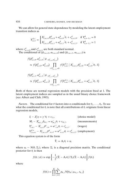
416 CARNEIRO, HANSEN, AND HECKMAN
We can allow for general state dependence by modeling the latent employment
transition indices as
Y d,∗
s,a,i
=
{ X
′
2,a,s,i
βa,s,0 d + αd ′
a,s,0 θi + εa,s,i,0 d , if Yd
s,a−1,i
= 0
X
2,a,s,i ′ βd a,s,1 + αd ′
a,s,1 θi + εa,s,i,1 d , if Yd
s,a−1,i
= 1
where εa,s,i,0 d and εd a,s,i,1
are both standard normal.
The conditional of (β 2,a,s,0 ,α 2,a,s,0 ) and (β 2,a,s,1 ,α 2,a,s,1 )is
f ( βa,s,0 d )
,αd ∣
a,s,0 ψ−β d
a,s,0 ,αa,s,0
d
∝ f ( βa,s,0 d ) ∏
,αd a,s,0 f ( Y d,∗
∣
s,a,i X
′
2,a,s,i βa,s,0 d + αd ′
a,s,0 θi , 1 )
i:Ys,a−1,i d =0
f ( βa,s,1 d )
,αd ∣
a,s,1 ψ−β d
a,s,1 ,αa,s,1
d
∝ f ( βa,s,1 d ) ∏
,αd a,s,1 f ( Y d,∗
s,a,i | X′ 2,a,s,i βd a,s,1 + αd ′
a,s,1 θi , 1 )
i:Ys,a−1,i d =1
Both of these are normal regression models with the precision fixed at 1. The
latent employment indices are sampled as in the usual binary choice framework
(see Albert and Chib, 1993).
Factors. The conditional for θ factors into n conditionals for θ 1 ,...,θ n . To see
what the conditional for θ i is note that all contributions of θ i originate from linear
regression models,
I i − Z
i ′ η = γ ′ θ i + ε I,i ,
(choice model)
M j − X
m,i, ′ j β m, j = α
m, ′ j θ i + ε m, j , (measurements)
Ys,a,i c − X′ 1,a,i βc s,a = α c s,a ′ θ i + εa,s,i c , (wages)
Y d,∗
2,s,a,i − X′ 2,a,s,i βd a,s,l = α d ′ a,s,l θ i + εa,s,i,l d , (employment)
This equation system is of the form
Ŷ i = A i θ i + u i
where u i ∼ N(0, i ), where i is a diagonal precision matrix. The conditional
posterior for θ i is then
{
f (θ i | ψ) ∝ exp − 1 }
2 (Ŷ i − A i θ i ) ′ i (Ŷ i − A i θ i ) f (θ i )
where
f (θ i ) =
K∏
J K ∑
k=1 j=1
p k, j N ( θ ik | µ k, j ,τ k, j
)