Diploma report Implementation and verification of a simple ... - LPAS
Diploma report Implementation and verification of a simple ... - LPAS
Diploma report Implementation and verification of a simple ... - LPAS

Create successful ePaper yourself
Turn your PDF publications into a flip-book with our unique Google optimized e-Paper software.
Figure 1: Illustration <strong>of</strong> a finite volume method where the average value Q ij is updated by<br />
the fluxes at the cell edges.<br />
which is a discrete approximation to the integral equation (22). The sum <strong>of</strong> the flux differences<br />
cancels out except for the fluxes at the extreme edges x I1 −1/2, x I2 +1/2, z J1 −1/2 <strong>and</strong><br />
z J2 +1/2. Therefore there will be exact conservation <strong>of</strong> the total quantity within the computational<br />
domain <strong>and</strong> this quantity will vary only due to the fluxes at the boundary.<br />
In order to obtain a fully discrete numerical method the second step is to discretize (23)<br />
in time. Some techniques <strong>of</strong> time integration will be discussed in section 3.4. One possibility<br />
<strong>of</strong> discretization is given here as an example <strong>and</strong> a fully discrete method is derived.<br />
Let ∆t = t n+1 − t n be the length <strong>of</strong> a time step, <strong>and</strong> let Q n ij represent the fully discrete<br />
approximation to Q ij (t n ). Then the time discretization <strong>of</strong> (23) is done by simply taking the<br />
difference between the values Q n+1<br />
ij<br />
<strong>and</strong> Q n ij <strong>and</strong> dividing by ∆t. The numerical method thus<br />
obtained has the form<br />
Q n+1<br />
ij<br />
= Q n ij − ∆t<br />
∆x (F i+1/2,j n − F i−1/2,j n ) − ∆t<br />
∆z (Gn i,j+1/2 − Gn i,j−1/2<br />
), (26)<br />
where the numerical fluxes Fi−1/2,j n <strong>and</strong> Gn i,j−1/2<br />
are some approximations to the time averages<br />
<strong>of</strong> the fluxes along the cell interfaces over the time interval [t n , t n+1 ]:<br />
Fi−1/2,j n ≈ 1 ∫ tn+1<br />
∫ zj+1/2<br />
f(q(x<br />
∆t∆z<br />
i−1/2 , z, t))dzdt,<br />
t n z j−1/2<br />
G n i,j−1/2 ≈ 1 ∫ tn+1<br />
∫ xi+1/2<br />
g(q(x, z<br />
∆t∆x<br />
j−1/2 , t))dxdt.<br />
t n x i−1/2<br />
(27)<br />
If these average fluxes can be computed based on the values Q n , then we will have a fully<br />
discrete method.<br />
For hyperbolic problems, information propagates with finite speed, so F n<br />
i−1/2,j <strong>and</strong> Gn i,j−1/2<br />
can be assumed to be based only on the cell averages on both sides <strong>of</strong> the interfaces x i−1/2<br />
10