Diploma report Implementation and verification of a simple ... - LPAS
Diploma report Implementation and verification of a simple ... - LPAS
Diploma report Implementation and verification of a simple ... - LPAS

Create successful ePaper yourself
Turn your PDF publications into a flip-book with our unique Google optimized e-Paper software.
x c = 0 m, x r = 4000 m, z c = 3000 m <strong>and</strong> z r =2000 m. The thermal perturbation has a<br />
minimum temperature <strong>of</strong> -15 ◦ C <strong>and</strong> is centered at x = 0 m <strong>and</strong> z = 3000 m. These initial<br />
conditions provide the negative buoyancy necessary to initiate a density current.<br />
The simulations are initiated with a thermal perturbation as described above <strong>and</strong> our<br />
model is integrated using Leapfrog <strong>and</strong> centered-in-space differences. Asselin <strong>and</strong> spatial<br />
filters are used to prevent oscillations in solutions. The value µ = 0.1 is chosen for all simulations,<br />
while ν is adjusted according to cells size <strong>and</strong> time step in order to always obtain a<br />
diffusion coefficient K <strong>of</strong> 75 m 2 s −1 , as this particular value is chosen for the reference problem<br />
in [8].<br />
Simulations are made using 80, 130 <strong>and</strong> 200 m resolution. According to [8], the flow features<br />
<strong>of</strong> the test problem should be adequately resolved for the first simulation <strong>and</strong> marginally<br />
resolved for the two others. The θ ′ solutions at 0, 300, 600 <strong>and</strong> 900 s from the three simulations<br />
are shown in Figure 13 <strong>and</strong> Figure 14.<br />
z[m]<br />
4000<br />
3000<br />
2000<br />
1000<br />
0<br />
80m<br />
t=0s<br />
z[m]<br />
4000<br />
3000<br />
2000<br />
1000<br />
0<br />
80m<br />
t=300s<br />
z[m]<br />
4000<br />
3000<br />
2000<br />
1000<br />
0<br />
80m<br />
t=600s<br />
z[m]<br />
4000 80m<br />
3000<br />
t=900s<br />
2000<br />
1000<br />
0<br />
0 2000 4000 6000 8000 10000 12000 14000 16000 18000<br />
x[m]<br />
Figure 13: Plots <strong>of</strong> θ’ at 0, 300, 600 <strong>and</strong> 900 s for the 80 m resolution solution.<br />
interval is 1 ◦ C <strong>and</strong> the contours are centered around 0 ◦ C.<br />
Contour<br />
Our model seems to be capable <strong>of</strong> correctly reproducing the basic characteristics <strong>of</strong> the<br />
flow in the test problem, even though the propagation speed <strong>of</strong> the density current is found<br />
to be slightly bigger in our model <strong>and</strong> the front <strong>of</strong> the perturbation ends a little further than<br />
in the reference model.<br />
In the solution from the 80 m resolution simulation, the three rotors are correctely reproduced.<br />
In the solution from the 130 m resolution simulation, the formation <strong>of</strong> the first<br />
rotor at 600 s is well reproduced. However, the third rotor is missing in the solution at 900 s.<br />
With 200 m resolution, the rotors are even less developed <strong>and</strong> there are significant quantitatives<br />
<strong>and</strong> qualitative differences between our solutions <strong>and</strong> the 25 m reference solution.<br />
36