Diploma report Implementation and verification of a simple ... - LPAS

More documents

Recommendations

Info

3.6.1 Gas dynamics (c = 1) A simple way to initialise the grid cells is to set ρ 0 = ρe 0 = 1 and ρu 0 = ρw 0 = 0. This initial conditions were used in particular during the different stages of model implementation in order to facilitate the verification of its functioning. 3.6.2 Unstratified atmosphere (g = 0) A more ”physical” but still unstratified atmosphere is initialised by setting ρ 0 equal to 1.25 kgm −2 in all grid cells. Lateral and vertical wind speed intensities u 0 and w 0 are then chosen and the initial momenta are given by the products ρ 0 u 0 and ρ 0 w 0 . To initialise the energy variable, a value for the temperature T 0 must also be specified an it is assumed to be constant in the whole domain. The energy is computed from ρe 0 = ρ 0 C v T 0 + 1 2 ρ 0(u 2 0 + w 2 0). (52) with ρe int = C v T where C v = 717 Jkg −1 K −1 is the specific heat at constant volume. 3.6.3 Stratified atmosphere (N = const) In the absence of atmospheric motion, there is a balance between vertical pressure gradient and buoyancy forces. In the atmosphere, the pressure of air decreases with increasing altitude. This creates an upward force, called the pressure gradient force. The force of gravity, on the other hand, almost exactly balances this out. Explicitly, hydrostatic balance is expressed as ∂p ∂z = −ρg. (53) The two variables, pressure and density, are related through the ideal gas law p = ρR d T, (54) where R d = 287 Jkg −1 K −1 is the gas constant for dry air. The temperature can be expressed as T = πθ, (55) where θ and π are the temperature and pressure that a parcel of dry air at temperature T and pressure p would have if it were brought at a standard pressure p s . θ is called the potential temperature and π the Exner function which is defined explicitely as π = ( p p s ) Rd /C p. (56) p s is the pressure at ground level and C p = 1004 Jkg −1 K −1 the specific heat at constant pressure. A last equation that is relevant for hydrostatic balance is N 2 = g θ where N is the buoyancy frequency usually taken to be 0.01 s −1 . ∂θ ∂z , (57) 17
In order to compute hydrostatic balance we need to express θ and π as functions of z only. θ(z) can be obtained by integrating equation (57) in z : ( N 2 ) θ(z) = θ s exp g z . (58) where θ s = θ(0). Substituting (54) in (53) and then writing this in terms of π and θ yields Integrating in z gives the equation for π π(z) = 1 − ∂π ∂z = − g C p θ . (59) g2 (1 − exp(−N2 z)), (60) C p θ s N 2 g and this equation is used to compute hydrostatic stratification. Then performing a backsubstitution T = πθ, p = p s π Cp/R d, ρ = R p d T , (61) ρe = γ − p 1 , yields the values for the components of q. 3.7 Boundary conditions In an atmospheric limited area model, only the lower boundary is physical. The other sides of the spatial domain are unbounded, meaning that the fluid flows in an exterior domain, and artificial boundaries must be introduced. In order to deal with the boundaries of the computational domain boundary conditions must be specified, for both artificial and physical boundaries. F n In the methods studied here, the value Q n ij is updated by computing the fluxes F n i−1/2,j , i+1/2,j , Gn i,j−1/2 and Gn i,j+1/2 . For doing that the neighboring cell values Qn i−1j , Qn i+1j , Qn ij−1 and Q n ij+1 are needed. But for the cells at the edges of the computational domain one or more of these values are missing. The general approach to this problem is to extend the computational domain to include a few additional cells, called ghost cells, on each side. 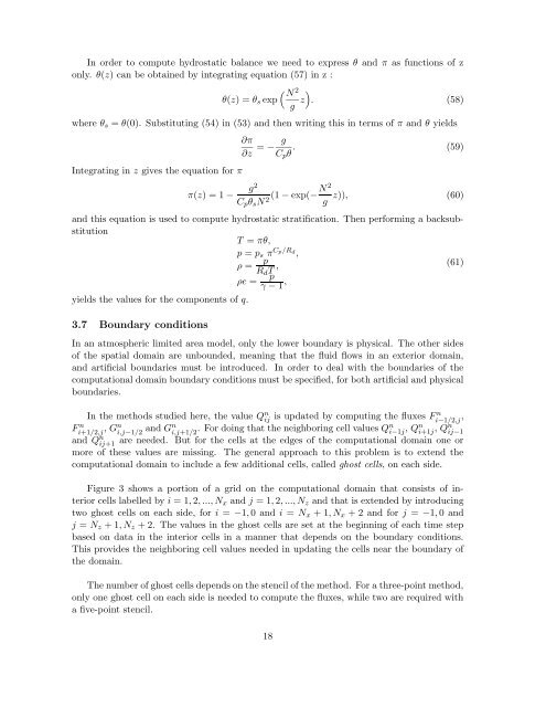Figure 3 shows a portion of a grid on the computational domain that consists of interior cells labelled by i = 1, 2, ..., N x and j = 1, 2, ..., N z and that is extended by introducing two ghost cells on each side, for i = −1, 0 and i = N x + 1, N x + 2 and for j = −1, 0 and j = N z + 1, N z + 2. The values in the ghost cells are set at the beginning of each time step based on data in the interior cells in a manner that depends on the boundary conditions. This provides the neighboring cell values needed in updating the cells near the boundary of the domain. The number of ghost cells depends on the stencil of the method. For a three-point method, only one ghost cell on each side is needed to compute the fluxes, while two are required with a five-point stencil. 18
Page 1: Diploma report Implementation and v
Page 4 and 5: 6 Acknowledgements 38 A Derivation
Page 6 and 7: In practice, however, many physical
Page 8 and 9: In developing the conservation laws
Page 10 and 11: and this expression can be used to
Page 12 and 13: and z j−1/2 respectively. They ca
Page 14 and 15: 3.3 Numerical fluxes There are diff
Page 16 and 17: 3.4.1 Forward Scheme The forward sc
Page 20 and 21: Figure 3: The lower left corner of
Page 22 and 23: π. In order to fill the ghost cell
Page 24 and 25: 4 Results 4.1 Comparison of differe
Page 26 and 27: time filter cst = 0 time filter cst
Page 28 and 29: in the (ij) grid cell is then s ij
Page 30 and 31: 400 t=0s 250 t=9s 350 200 300 150 2
Page 32 and 33: 4.4 Advection Advection of a densit
Page 34 and 35: 1000 u’ ∆x=∆z=25m t=100s 800
Page 36 and 37: 4.5 Buoyant bubble In order to stud
Page 38 and 39: 4000 4000 z[m] 3000 2000 1000 0 130
Page 40 and 41: A Derivation of the differential fo

Diploma report Implementation and verification of a simple ... - LPAS

You also want an ePaper? Increase the reach of your titles

Delete template?

Save as template?