Get my PhD Thesis

J. Chem. Phys., Vol. 121, No. 1, 1 July 2004 Self-consistent field method
19
where i HOMO () and a LUMO () are the HOMO and LUMO
orbital energies, respectively; in Fig. 1b, we have plotted
the overlap between the old and new density matrices as
given by
DD¯ S
a
,
DDS D¯D¯ S
22
where D()D() S is equal to N/2. For sufficiently large
, the HOMO-LUMO gap Eq. 21 is linear in . This linearity
of ai () for large arises from the dependence of
the orbital energies on in Eq. 19, where is effectively
subtracted from the occupied orbital energies. The MOs C¯occ
occupied in D¯ satisfy the generalized eigenvalue equations
SD¯SC¯occ SC¯occ ,
23
and become identical to the MOs C occ () obtained from Eq.
19 when tends to infinity. The corresponding density is
denoted
T
DC¯occ C¯occ
24
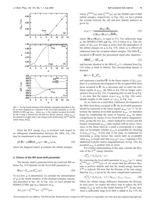
FIG. 1. For the fourth iteration of the rhodium calculation described in Sec.
III we have displayed as a function of the level-shift parameter ; a the
HOMO-LUMO gap ai , where min is the smallest accepted level-shift,
b the overlap a between the old and new density matrices, where opt is
the optimal level-shift, and c the change in the model energy E RH and the
actual energy E RH SCF .
Since the SCF energy E SCF is invariant with respect to
an orthogonal transformation between the MOs, Eq. 18
may be transformed to the canonical basis:
FD¯SD¯SC occ SC occ ,
where the diagonal matrix contains the orbital energies.
2. Choice of the RH level-shift parameter
19
The density matrix generated from the restricted RH solution
Eq. 19 depends on the level-shift parameter :
DC occ C T occ . 20
To see how is determined, we consider the determination
of in the fourth iteration of the rhodium-complex calculation
described in Sec. III. In Fig. 1a, we have plotted the
HOMO-LUMO gap as a function of ,
ai a LUMO i HOMO ,
21
and represents a purified D¯. In the linear regime of ai (),
there is a continuous development of the occupied MOs from
those occupied in D¯. As decreases and we enter the nonlinear
regime at min , the MOs in Eq. 20 no longer correspond
to those in Eq. 23. Comparing plot a and b in Fig.
1, we note that the region a()a min in Fig. 1b corresponds
roughly to the region min in Fig. 1a.
As we insist on a controlled, continuous development of
the MOs from those occupied in D¯, the level-shift parameter
should be restricted to the linear regime min . To determine
the optimal level-shift parameter opt , we therefore
begin by establishing the onset of linearity min by linear
extrapolation by means of two Fock/KS matrix diagonalizations,
giving the two ai values marked by crosses and the
linearly interpolated min value marked with an arrow. Next,
since, in the linear interval, a small corresponds to a large
step, we investigate whether min is acceptable by checking
if a( min )a min . If this step is too long, we backtrack by
increasing using inexact line search until an acceptable
value opt is found such that a( opt )a min , requiring a few
additional Fock/KS matrix diagonalizations. In Fig. 1b, the
accepted opt is marked with an arrow.
For a better understanding of this step, consider the Hessian
of the E RH energy function:
A RH ai,bj ij ab a i . 25
By restricting the level-shift parameter to min where
LUMO a () HOMO i ()0, we ensure that the effective Hessian
is positive definite and that the model energy function
E RH is reduced. We note that the Hessian of the true energy
function E SCF is given by the more complicated expression
A SCF ai,bj ij ab a i 4g aibj g abij g ajib . 26
Often, the orbital energy difference dominates the Hessian.
In such cases, we expect the above step to reduce the SCF
energy E SCF as well as the model function E RH . In any case,
when a sufficiently large level shift is added in Eq. 19, the
Downloaded 25 Jun 2004 to 130.225.22.254. Redistribution subject to AIP license or copyright, see http://jcp.aip.org/jcp/copyright.jsp