Get my PhD Thesis

Part 2
Atomic Orbital Based Response Theory
the linear response function in Eq. (2.42) can be obtained as
[1]
B
AB ; ω
=−A N ( ω)
. (2.44)
2.2.5 Pairing
The excitation energies are identified as the poles of the linear response function of Eq. (2.42) and
are therefore solutions to the generalized eigenvalue problem
[2] [2]
E X = ωS X. (2.45)
In the MO formulation of response theory, it has been shown that the excitation energies are
paired 63 , so that if ω i is an eigenvalue for Eq. (2.45) then so is -ω i . It is important to understand how
pairing appears in the AO basis, in particular since this structural feature is exploited when the
equations are solved iteratively as is necessary for large problems. This is further discussed in
Section 2.3. Since the proof of the pairing given in the MO formulation cannot be directly
transferred to the AO formulation due to the presence of the diagonal operators D m , this section
gives the proof in the AO formulation.
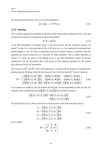
The structure of E [2] and S [2] in the AO formulation is analyzed for the purpose of examining the
pairing structure. Dividing Λ into the tree classes of Eq. (2.28), the matrix E [2] may be written as
†
⎛ 0 ⎡⎣Q, ⎡⎣H0, Q ⎤⎤ ⎦⎦ 0 0 [ Q, [ H0, D]
] 0 0 [ Q, [ H0, Q]
] 0 ⎞
[2]
⎜
⎟
†
E = ⎜ 0 ⎣⎡D, ⎣⎡H0, Q ⎦⎦ ⎤⎤ 0 0 [ D, [ H0, D]
] 0 0 [ D, [ H0, Q]
] 0 ⎟. (2.46)
⎜ † † † †
⎟
⎝ 0 ⎣⎡Q , ⎣⎡H0, Q ⎦⎦ ⎤⎤ 0 0 ⎣⎡Q ,[ H0, D] ⎦⎤ 0 0 ⎣⎡Q ,[ H0, Q]
⎦⎤
0 ⎠
If we assume for simplicity that all orbitals and integrals for the unperturbed system are real, the
†
elements of for example the block 0 ⎡⎣Q ,[ H0
, Q ] ⎤⎦
0 are trivially rewritten as
† †
∗
0 ⎡⎣Qm, [ H0, Qn ] ⎤⎦ 0 = 0 ⎡⎣Qm, [ H0, Qn
] ⎤⎦
0
(2.47)
†
= 0 ⎡⎣Qm, ⎡⎣H0
, Qn
⎤⎤ ⎦⎦ 0 .
The nine blocks in Eq. (2.46) can then all be written in terms of the following four matrices
and we obtain
†
mn m 0 n
A = 0 ⎡⎣Q , ⎡⎣H , Q ⎤⎤ ⎦⎦ 0 ,
Bmn = 0 ⎡⎣Qm , ⎡⎣H0
, Qn
⎤⎤ ⎦⎦ 0 ,
(2.48)
Fmn = 0 ⎡⎣Qm , ⎡⎣H0
, Dn
⎤⎤ ⎦⎦ 0 ,
Gmn = 0 ⎡⎣Dm , ⎡⎣H0
, Dn
⎤⎤ ⎦⎦ 0 ,
⎛ A F B ⎞
[2] ⎜ T T
E = F G F
⎟
. (2.49)
⎜
⎟
⎝ B F A ⎠
66