Get my PhD Thesis

Part 2
Atomic Orbital Based Response Theory
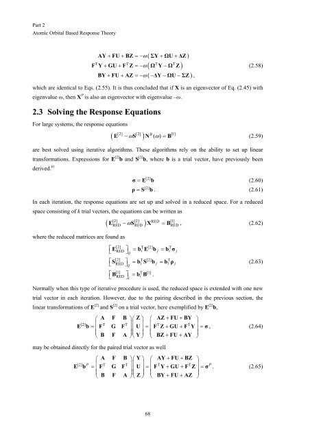
AY + FU + BZ = − ω ( ΣY + ΩU + ∆Z )
( )
T T T T
F Y+ GU+ F Z = −ω
Ω Y −Ω Z
BY + FU + AZ = −ω
( −∆Y −ΩU −ΣZ
),
(2.58)
which are identical to Eqs. (2.55). It is thus concluded that if X is an eigenvector of Eq. (2.45) with
eigenvalue ω, then X P is also an eigenvector with eigenvalue –ω.
2.3 Solving the Response Equations
For large systems, the response equations
( ω )
[2] [2] [1]
E − S N B ( ω ) = B (2.59)
are best solved using iterative algorithms. These algorithms rely on the ability to set up linear
transformations. Expressions for E [2] b and S [2] b, where b is a trial vector, have previously been
derived. 61 [2]
σ = E b (2.60)
[2]
ρ = S b. (2.61)
In each iteration, the response equations are set up and solved in a reduced space. For a reduced
space consisting of k trial vectors, the equations can be written as
where the reduced matrices are found as
( ω )
[2] [2] RED [1]
RED
−
RED
=
RED
E S X B , (2.62)
[2] T [2] T
RED ⎦ i j i j
ij
⎡
⎣
E ⎤ = b E b = b σ
[2] T [2] T
RED ⎦ i j i j
ij
⎡
⎣
S ⎤ = b S b = b ρ
[1] T [1]
RED ⎦
bi
B .
i
⎡
⎣
B ⎤ =
(2.63)
Normally when this type of iterative procedure is used, the reduced space is extended with one new
trial vector in each iteration. However, due to the pairing described in the previous section, the
linear transformations of E [2] and S [2] on a trial vector, here exemplified by E [2] b,
⎛ A F B ⎞⎛ Z⎞ ⎛ AZ+ FU+
BY ⎞
[2] ⎜ T T ⎟⎜ ⎟ ⎜ T T
E b = F G F U = F Z+ GU+ F Y
⎟
= σ , (2.64)
⎟⎜ ⎜ ⎟⎜ ⎟ ⎜
+ +
⎟
⎝ B F A ⎠⎝Y⎠ ⎝ BZ FU AY ⎠
may be obtained directly for the paired trial vector as well
⎛ A F B ⎞⎛Y⎞ ⎛ AY+ FU+
BZ ⎞
[2] P ⎜ T T ⎟⎜ ⎟ ⎜ T T ⎟ P
E b = F G F U = F Y+ GU+ F Z = σ . (2.65)
⎟⎜ ⎜ ⎟⎜ ⎟ ⎜
+ +
⎟
⎝ B F A ⎠⎝ Z⎠ ⎝ BY FU AZ ⎠
68