Get my PhD Thesis

Part 1
Improving Self-consistent Field Convergence
F orth
R
λ min
Estimate and
for F orth
λ max
0
orth
( λ
max
I
−
F
)
=
( λ
−
λ
)
max
min
1
x n +1 = 2x n - x n
2
n = n + 1
Tr Rn > N
yes
R
n+ 1 =
R
2
n
no
2
n+ 1 = 2 n − n
R R R
x n +1
no
Tr Rn N ε
+ 1 − <
yes
D orth = R n+1
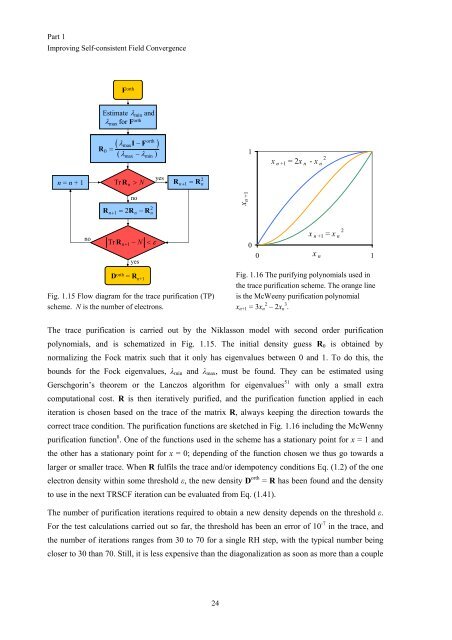
Fig. 1.15 Flow diagram for the trace purification (TP)
scheme. N is the number of electrons.
0
x n +1 = x n
2
0 x n
1
Fig. 1.16 The purifying polynomials used in
the trace purification scheme. The orange line
is the McWeeny purification polynomial
x n+1 = 3x n 2 – 2x n 3 .
The trace purification is carried out by the Niklasson model with second order purification
polynomials, and is schematized in Fig. 1.15. The initial density guess R 0 is obtained by
normalizing the Fock matrix such that it only has eigenvalues between 0 and 1. To do this, the
bounds for the Fock eigenvalues, λ min and λ max , must be found. They can be estimated using
Gerschgorin’s theorem or the Lanczos algorithm for eigenvalues 51 with only a small extra
computational cost. R is then iteratively purified, and the purification function applied in each
iteration is chosen based on the trace of the matrix R, always keeping the direction towards the
correct trace condition. The purification functions are sketched in Fig. 1.16 including the McWenny
purification function 8 . One of the functions used in the scheme has a stationary point for x = 1 and
the other has a stationary point for x = 0; depending of the function chosen we thus go towards a
larger or smaller trace. When R fulfils the trace and/or idempotency conditions Eq. (1.2) of the one
electron density within some threshold ε, the new density D orth = R has been found and the density
to use in the next TRSCF iteration can be evaluated from Eq. (1.41).
The number of purification iterations required to obtain a new density depends on the threshold ε.
For the test calculations carried out so far, the threshold has been an error of 10 -7 in the trace, and
the number of iterations ranges from 30 to 70 for a single RH step, with the typical number being
closer to 30 than 70. Still, it is less expensive than the diagonalization as soon as more than a couple
24