analytical solution for one-dimensional semi-infinite heat - LEPTEN

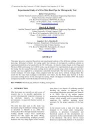
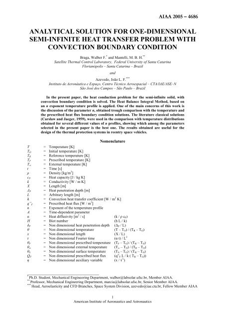
AIAA 2005 – 4686
ANALYTICAL SOLUTION FOR ONE-DIMENSIONAL
SEMI-INFINITE HEAT TRANSFER PROBLEM WITH
CONVECTION BOUNDARY CONDITION
Braga, Walber F. * and Mantelli, M. B. H. **
Satellite Thermal Control Laboratory, Federal University of Santa Catarina
Florianópolis – Santa Catarina – Brazil
and
Azevedo, João L. F. ***
Instituto de Aeronáutica e Espaço, Centro Técnico Aeroespacial – CTA/IAE/ASE–N
São José dos Campos – São Paulo – Brazil
In the present paper, the heat conduction problem for the semi-infinite solid, with
convection boundary condition is solved. The Heat Balance Integral Method, based on
an n exponent temperature profile is applied. One of the main concerns of this work is
the discussion of the parameter n, obtained trough comparison with the temperature and
the prescribed heat flux boundary condition solutions. The literature classical solutions
(Carslaw and Jaeger, 1959), were used in the comparison with temperature distributions
obtained for several different values of n profiles, showing which among the parameters
selected in the present paper is the best one. The results obtained are useful for the
design of the thermal protection systems in reentry space vehicles.
Nomenclature
T = Temperature [K]
T O = Initial temperature [K]
T R = Reference temperature [K]
T F = Prescribed temperature [K]
T ∞ = External temperature [K]
t = Time [s]
ρ = Density [kg/m 3 ]
c P = Heat capacity [J / kg K]
k = Conductivity [W / m K]
X = Length [m]
∆ P = Heat penetration depth [m]
L = Arbitrary length [m]
h = Convection heat transfer coefficient [W / m 2 K]
q” F = Prescribed heat flux [W / m 2 ]
n = Exponent of the temperature profile
A = Time-dependent parameter
α = Heat diffusivity [m 2 / s] (k / ρ c P )
H = Biot number (h L / k)
δ P = Non dimensional heat penetration depth (∆ P / L)
θ = Non dimensional temperature (T – T O ) / (T R – T O )
x = Non dimensional length (X / L)
τ = Non dimensional Fourier time (α t) / L 2
θ F = Non dimensional prescribed temperature (T F – T O ) / (T R – T O )
θ ∞ = Non dimensional external temperature (T ∞ – T O ) / (T R – T O )
θ S = Non dimensional surface temperature (T S – T O ) / (T R – T O )
Q F = Non dimensional prescribed heat flux (q” F L / k ( T R – T O ))
η = Non dimensional auxiliary variable (x / τ ½ )
______________________________________
* Ph.D. Student, Mechanical Engineering Department, walber@labsolar.ufsc.br, Member AIAA.
** Professor, Mechanical Engineering Department, marcia@labsolar.ufsc.br, Senior Member AIAA.
*** Head, Aeroelasticity and CFD Branches, Space System Division, azevedo@iae.cta.br, Fellow Member AIAA
1
American Institute of Aeronautics and Astronautics

I. Introduction
Conduction heat transfer is a very important phenomenon to the engineering science. Since the Fourier’s
work “La Théorie Analytique de la Chaleur”, many mathematics methods has been developed to assist modern
engineers, helping them to understand and predict the thermal behavior of different problems. Even being one of
the most studied subjects on the thermal engineering field, heat conduction is still an interesting phenomenon
with many challenging problems that still need to be solved. Some examples of these unsolved problems can be
found within a material undergoing ablation, due to an imposed heat flux or temperature in its external free
surface, as it happens in the thermal protection materials of reentry spacecrafts and satellites.
The authors of the present paper have being studying analytically the heat conduction and ablation problems
using the electrical analogy (Braga et al. 2002) 1 and the Heat Balance Integral Method (HBIM). Braga et al.
(2003) 2 studied the semi-infinite conduction problem, using the HBIM, subjected to the prescribed time-variable
heat flux boundary condition in its free surface. This same authors (Braga et al., 2004) 3 studied this same
problem, subjected to the free surface time-constant heat flux boundary condition in a finite solid with an
insulated opposite surface. In both papers, the pre-ablation and ablation phases were considered. From these
previous works, it was observed the need to better understand the effect of the selected temperature profiles used
at the HBIM on the accuracy of the obtained solution.
As it will be described later, in all these problems the solid is subjected to pure conduction heating process,
before undergoing the ablation. Table 1 shows the combination of some possible heat conduction problems for
the pre-ablation period, according to the boundary conditions applied. In this Table, the left two columns
represent the boundary conditions applied on the right side of the solid, which can be considered semi-infinite or
finite. For the finite case, the following boundary conditions can be considered: prescribed temperature (PT),
prescribed heat flux (PH) or convection (C). The last three columns of Table 1 represent the free surface on the
left side of the domain, which will be ablated after the appropriate temperature level is achieved (the ablation
will not be considered in the present paper). The left surface can, in turn, be subjected to the same boundary
conditions. All the possible combinations can be found in this table. The cases marked with an ∆ in the table
were presented at previous work (Braga et al. 2005) 7 . Only the X marked case is considered in the present work,
but the methodology presented can be used to solve all the remaining cases. Figure 1 illustrates the heat
conduction problem for the semi infinite and finite solid with the three mentioned left and right boundary
conditions (PT, PH and C).
The Heat Balance Integral Method (HBIM), as presented by Goodman (1964) 4 , is used in the analytical
solution of the present cases. In this method, an n exponent temperature profile is assumed for the temperature
distribution. The precision of the method is directly related to the correct choice of this parameter. In the present
paper, a procedure used to select the appropriate n parameter is presented.
Analyzing the thermal behavior of a heated solid, it can be noted that, in the pre-ablation problems and, at
the very first moment, the temperature profile is the same of that obtained for a simple problem without
ablation. As the time goes on, the temperature increases, starting the ablation. As a consequence, the
temperature profile changes and, in the limit, as time goes to infinity, it tends to that observed for a surface
prescribed temperature (without ablation) problem. Therefore, one can conclude that a good choice of the profile
exponent n should be a time dependent parameter, able to capture the transition between these limiting curves.
Semi-finite Solid
T P
q” F
or
h,
T ∞
or
Finite Solid
T P
h,
T ∞
or
q” F
or
h,
T ∞
or
q” F
or
T P
Figure 1. Graphic representation of the possible heat conductions problems.
2
American Institute of Aeronautics and Astronautics

Table 1. Possible pre-ablation problems according to the applied boundary conditions.
Left free surface boundary condition
PT PH C
Semi-infinite ∆ ∆ X
Right boundary
condition
Finite – PT
Finite – PH
Finite - C
In the present paper, the Heat Balance Integral Method is used to solve the heat conduction problems for a
semi-infinite solid without ablation using a time variable exponent temperature profile n, with a time constant
convection boundary condition.
II.
Physical Modeling
The case of a one dimensional semi-infinite solid body made of an isotropic material with constant
properties is considered. The body is assumed to be at a constant initial temperature until the start up of the
heating process, by convection on its surface. A heat transfer coefficient (H) and a constant reference
temperature (θ ∞ ) are assumed. The heat is conducted inside the material, developing two different sections: the
heated region, which the temperature is affected by the surface imposed heat and the virgin region where the
material has not felt the presence of the surface heating, remaining at the initial temperature. The distance
between the surface of the material and the front end of the regions is named as the heat penetration depth (δ P ).
Figure 2 shows the physical model scheme adopted for the case under analysis.
θ ∞
H
Heated
Region
Virgin
Material
x
δ P
Figure 2. Physical modeling scheme.
III.
Mathematical Modeling
In this section, the mathematical models used to predict the thermal behavior of the problems considered are
developed.
A heat balance over the body (see Fig. 2) leads to the following well known transient non-dimensional
differential heat equation, where θ=(T –T O )/(T R –T O ), T O is the initial temperature and T R is any arbitrary
reference temperature:
2
=
2
x
.
(1)
In this equation, τ is the Fourier non dimensional time, defined as τ = (α t)/L 2 , where α is the heat diffusivity,
t is the time and L corresponds to an arbitrary length. Also, x is defined as x = X / L, where X is the dimensional
length.
The following boundary conditions are considered for these problems. If there is not a virgin region in the
material, i.e., if all the solid material already experiences the presence of the heating imposed at the surface, the
boundary condition considered for the right edge located at the infinity is:
lim = 0
x
lim =
and 0 .
x x
(2)
3
American Institute of Aeronautics and Astronautics

If there is a virgin region, i.e., if the time is not enough for the heat to reach the entire solid, the boundary
conditions, located in the border line between the heated and the virgin regions, are:
= 0 and = 0
x= P
x
x= P
.
(3)
At the free surface of the material, the convection boundary is given by:
x
x=
0
= H
(
)
x=
0
.
(4)
IV.
Solutions
In this section, the problem under investigation will be solved, using two different analytical methods.
A. Classical Solution
The classical solutions found in the literature are obtained using the Laplace Transform technique or using a
variable transformation, as presented by many of the classical conduction heat transfer books, such as Arpaci
(1966) 5 , Carslaw and Jaeger (1959) 6 , among others. These solutions are reproduced for the problem under
analyzes, as follows.
For the constant heat flux at the free surface case, the solution of the partial differential equation (Eq. 1)
subjected to the boundary conditions given by Eqs. 2 and 4 is:
( )
x
2 x
=
erfc
+
exp H x H erfc
+ H
2
2
.
(5)
The Duhamel’s theorem needs to be used to obtain the solution for a variable convection boundary condition
on the free surface, when needed.
B. Heat Balance Integral Method
The Heat Balance Integral Method (HBIM) is based on the integral form of the heat conduction differential
equation. This form is obtained by the integration of Eq. 1 with respect at the position x, from the solid surface
(x=0) up to the heat penetration depth, (x=δ P ). Doing so, the following equation is obtained:
P
dx =
x x
0 x= P x=0
. (6)
As δ P is a time-dependent variable, the Leibniz rule is used and the Eq. 6 is rearranged as:
d
d
P
d
P
dx
=
x= P
0 d
x x
x=
x=0
P
. (7)
At this point, an appropriate function has to be selected as the profile of the temperature distribution inside
the material. This function must have a good agreement with the space boundary conditions and must present
time dependent parameters, which are determined using the remaining initial condition. In this paper, the
following profile is considered:
P
x
A
=
P
n
, (8)
4
American Institute of Aeronautics and Astronautics

where A is the time-dependent parameter, calculated through the free surface boundary condition and represents
the surface temperature. Physically, this parameter represents the surface temperature of the material, while n
establishes the shape of the temperature profile along the solid, being arbitrarily selected. The best selection of
the n value and its implications will be explained latter on this paper. The profile represented by Eq. 8 naturally
satisfies the boundary conditions given by Eq. 3. Substituting Eq. 8 in Eq. 7 one gets the following ordinary
differential equation:
d A
P
d
An
=
( n )
P
+1 . (9)
The prescribed heat flux problem is solved in this section. The temperature distribution (Eq. 8) is substituted
in the convection boundary condition (Eq. 4), obtaining the following equation:
An
P
= H
( A )
.
(10)
Solving for A, one gets:
H
P
A = n
H
+
P
n
1 .
(11)
Substituting Eq. 11 in Eq. 9 the following differential equation is obtained:
H
P
H
P
d
n
P
= n
d H
+
+
P
1
n
n
( n + 1) H
P P
1 .
n
(12)
This equation can be solved for the heat penetration depth, resulting in:
( n + 1)
n
= 1,
exp
2 H 2
P
LambertW
1 1
H
n
, (13)
which LambertW(-1, x) is the second order branch of the LambertW(x) equation. Note that all parameters H, θ ∞
and n are considered time constant in this solution. Summarizing, the temperature profile is given by Eq. 8, the
surface temperature by Eq. 11 and the heat penetration depth (δ P ) by Eq. 13. Therefore, the only unknown
variable is the n parameter.
C. Comparison between the solutions obtained through the Heat Balance Integral Method
The same temperature profile (Eq. 8) is adopted in the present development and in previous work (Braga et
al. 2005) 7 enabling the solutions to be compared. Table 2 presents the results obtained by Braga et al. (2005) 7 .
The n parameter (last line of Table 2) was deeply discussed in this paper.
Just as a study case, the following configurations will be compared: prescribed heat flux with Q = 1,
prescribed temperature with θ F = 1, and finally, convection with H = 1 and θ ∞ = 1. For all three cases the same
n value is 2,5, due the fact that the presented solutions are highly dependent on the choice of n. Figure 3 presents
the heat penetration depth and the non dimensional surface temperature as a function of time for plots all the
three cases.
5
American Institute of Aeronautics and Astronautics

Surface Temperature
Heat Penetration Depth
Heat Penetration Depth
(constant n value)
Heat Penetration Depth
Table 2. Summary of the previous HBIM solutions.
Prescribed Heat Flux
Prescribed Temperature
P
P
=
=
A
Q
n
F
P
= A =
F
( n + 1)
n
Q
F
0
( n + 1)
n
Q
F
0
Q
Q
F
F
d
d
P
=
P
=
2
( n + 1)
2
F
2 n
2
n
+
0
( n 1)
( n + 1) 2
= n
(constant n, Q F and θ F
( n + 1)
values) P
P
= 2 n( n + 1)
2
Optimum n parameter n = 3,66
n = 1,75
4
2
( )
F
( )
0
2
F
2
F
d
d
Legend:
Figure 3. Comparison between the HBIM solutions.
At the Fig. 3 can be noted that the convection solution begins exactly as a prescribed heat flux solution and it
tends to the prescribed temperature ones as the time goes on. It is physically explained as the following: at the
very beginning, the surface temperature is equal to zero then it is suddenly exposed to a convection situation
which is like to expose the surface at a prescribed heat flux defined as Q = H θ ∞ . As time goes to infinity there is
very few changes at the surface temperature since it is already almost equal to the external temperature, θ ∞ . So,
physically, the convection solution is a blending solution between the prescribed heat flux and the prescribed
temperature solutions. The problem is that different optimum n values where obtained for each kind of solution.
V. Obtaining the parameter n
As described before, the n parameter is the exponent of the temperature distribution profile adopted and,
generally, is arbitrarily selected. Usually, this profile has an exponential function shape, which satisfies the Eq. 2
boundary conditions, or a polinomium, that instead, satisfies the boundary conditions expressed by Eq. 3. In the
present work, the n value is free to attain any real decimal value and to vary with time. Goodman (1964) 4
presents the error (difference between classical and HIBM solutions, divided by classical solution) for some
polinomium with different degrees. This author showed that the surface temperature for the prescribed heat flux
condition presents large error for n = 2 (8,6%), which decreases for n = 3 (2,0%) but there is no guarantee that
increasing the order of the polynomial will improve the accuracy.
To find out the best value for n, the classical solution, which is exact, can be used. The strategy usually
adopted is to perform an energy balance in the solid, using both the classical and the HBIM solutions. The total
energy in these cases should be the same. In the present work this procedure is not possible due the fact that,
during the solution of the problem, the n parameter was assumed to be a constant value and the total energy
method indicates a time variable solution to the n. Therefore, in this work, an average value of n was adopted,
between the optimums n of the prescribed heat flux and of the prescribed temperature problems:
6
American Institute of Aeronautics and Astronautics

n =
2
+
1
( 4
) ( 2)
2,7
.
(14)
VI.
Comparison between the Classical Solution and the Heat Balance Integral Method
The comparison between the classical and the HBIM solutions is made using the temperature profiles (Eqs. 5
and 15) and the surface temperatures (Eq.16 and Eq.17). This comparison is based on the problem: H = 1 and θ ∞
= 1.
= 1
1
( n + 1)
2
( n )
LambertW
H
+ 1 2
1,
exp 2 1
1,
exp 2 H 1
1
1
n
n
LambertW
x H
n
n
(15)
S
= 1
( n + 1)
1,
exp 2 H 2
1
S
LambertW
1
2
( 1 exp( H ) erfc ( H
)
=
.
n
.
(16)
(17)
Figure 4 presents the plots of the normalized temperature with respect to the surface temperature (θ / θ S ) as a
function of the parameter η, defined as (η = x / τ ½ ). The graphic shows the classical solution (given by Eq. 5)
and the others using the HIBM solutions (given by Eq. 15 and Table 2), considering different values of the
parameter n (2, 2.7 and 3) and different τ values. In Fig. 5, the absolute error for the HBIM (defined as ε ABS =
Eq. 5/ Eq. 17 – Eq. 15/ Eq. 16) is presented for the different n values.
It can be noted in Fig. 4 that the temperature distribution curves for n = 2,7, n = 3 and the classical solution
present very similar shapes, being hard to distinguish among them. In Fig. 5, the absolute errors curves for the
cases n = 2,7 and n = 3 have similar behavior, but the curve for n = 2,7 shows the minimum error levels, being
the best choice among all the cases studied. It is interesting to note again the transitory behavior of the
convection solution which goes from the prescribed heat flux solution for small τ values to the prescribed
temperature solution for larger values.
7
American Institute of Aeronautics and Astronautics

n = 2 n = 2,7 n = 3
τ = 100
τ = 10
τ = 0.01
Legend:
Figure 4. Normalized temperature profiles.
n = 2 n = 2,7 n = 3
Figure 5. Normalized temperature absolute errors.
8
American Institute of Aeronautics and Astronautics

The relative error ε for the prediction of the surface temperature can be obtained through Eq. 16 and Eq. 17
(1 – Eq. 16/ Eq. 17), resulting in:
1
= 1
LambertW 1,
exp
2
( n + 1)
2
( 1
exp( H ) erfc ( H
)
1
n
H
2
1
, (18)
Figure 6 presents the graphic of this error against the n parameter and the Fourier time ( τ ), using Eq. 18. It
can be observed in these figures that the error depends on the n value as well as on the time. It means that a good
accuracy of the surface temperature results using the HBIM depends on the time and on the value of n.
n
n
Figure 6. Relative error of the surface temperature against the n parameter and the Fourier time (τ)
VII.
Conclusion
In this paper the Heat Balanced Integral Method was used to solve the heat conduction inside a semi-infinite
solid body subjected to a time constant convection boundary condition. As part of the method, an n degree
function was selected as representative of the temperature distribution of the material.
The value of the n exponent (Eq. 8) was selected based on the temperature distribution obtained from the
classical solution temperature distribution profile, which was compared with other n values. The comparison
shows that the value of n = 2,7 is good to be used in these problems.
It is important to note that the best value of n is very dependent on the physical behavior of the problem. Due
to this fact, the authors believe that a time-constant n value is not the best choice to the convective boundary
condition problem.
The present case as well the others mentioned in Table 1, which were not studied in the present work, needs
to be better investigated. As already mentioned in the Introduction section, a constant value of the parameter n
was adopted in former previous modeling developed by the authors, which included ablation. The methodology
presented in this paper should be used to improve the other results previously published in the literature.
References
1 Braga, W.F., Mantelli, M.B.H., “Electrical Analogy Modeling for One-Dimensional Ablation Problem”, 8 th
AIAA/ASME Joint Thermophysics and Heat Transfer Conference, Saint Louis, AIAA, 2002.
2 Braga, W.F., Mantelli, M.B.H., Azevedo, J.L.F., “Approximated Analytical Solution for One-Dimensional
Ablation Problem with Time-Variable Heat Flux”, 36 th AIAA Thermophysics Conference, Orlando, AIAA,
2003.
3 Braga, W.F., Mantelli, M.B.H., Azevedo, J.L.F., “Approximate Analytical Solution for One-Dimensional
Finite Ablation Problem with Constant Time Heat Flux”, 37 th AIAA Thermophysics Conference, Portland,
AIAA, 2004.
9
American Institute of Aeronautics and Astronautics

4 Goodman, T.R., “Application of Integral Methods to Transient Nonlinear Heat Transfer”, Advances in Heat
Transfer, Vol. 1, Academic Press, New York, 1964, pp. 51-122.
5 Arpaci, V.S., “Conduction Heat Transfer”, Addison-Wesley, Menlo Park, 1966.
6 Carslaw, H.S., Jaeger, J.C., “Conduction of Heat in Solids”, 2 nd ed., Oxford University Press, London,
1959.
7 Braga, W.F., Mantelli, M.B.H., Azevedo, J.L.F., “A New Approach for the Heat Balance Integral Method
Applied to Heat Conduction Problems”, 43 rd AIAA Aerospace Sciences Meeting and Exhibit, Reno, AIAA,
2005.
10
American Institute of Aeronautics and Astronautics