Agricultural Drought Indices - US Department of Agriculture
Agricultural Drought Indices - US Department of Agriculture
Agricultural Drought Indices - US Department of Agriculture

Create successful ePaper yourself
Turn your PDF publications into a flip-book with our unique Google optimized e-Paper software.
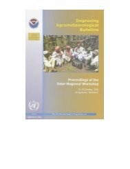
<strong>Agricultural</strong><br />
<strong>Drought</strong> <strong>Indices</strong><br />
Proceedings <strong>of</strong> an<br />
expert meeting<br />
2–4 June 2010, Murcia, Spain<br />
World Meteorological<br />
Organization<br />
United States<br />
<strong>Department</strong> <strong>of</strong> <strong>Agriculture</strong><br />
World <strong>Agricultural</strong><br />
Outlook Board<br />
National <strong>Drought</strong><br />
Mitigation Center<br />
United Nations<br />
International Strategy for<br />
Disaster Reduction<br />
Government <strong>of</strong> Spain Ministry<br />
for<br />
Environmental, Rural<br />
and Marine Affairs<br />
Hydrographic<br />
Confederation <strong>of</strong> Segura
<strong>Agricultural</strong> <strong>Drought</strong> <strong>Indices</strong><br />
________________________________________________________________________<br />
Proceedings <strong>of</strong> an Expert Meeting<br />
2-4 June, 2010, Murcia, Spain<br />
Editors<br />
Mannava V.K. Sivakumar<br />
Raymond P. Motha<br />
Donald A. Wilhite<br />
Deborah A. Wood<br />
Sponsors<br />
World Meteorological Organization<br />
United Nations International Strategy for Disaster Reduction (UNISDR)<br />
Hydrographic Confederation <strong>of</strong> Segura, Spain<br />
United States <strong>Department</strong> <strong>of</strong> <strong>Agriculture</strong><br />
National <strong>Drought</strong> Mitigation Center<br />
University <strong>of</strong> Nebraska, Lincoln, Nebraska, <strong>US</strong>A<br />
AGM-11<br />
WMO/TD No. 1572<br />
WAOB-2011<br />
World Meteorological Organization<br />
7bis, Avenue de la Paix<br />
1211 Geneva 2<br />
Switzerland<br />
2011
© World Meteorological Organization, 2011<br />
The right <strong>of</strong> publication in print, electronic, and any other form and in any language is reserved by<br />
WMO. Short extracts from WMO publications may be reproduced without authorization provided<br />
that the complete source is clearly indicated. Editorial correspondence and requests to publish,<br />
reproduce or translate this publication (articles) in part or in whole should be addressed to:<br />
Chairperson, Publications Board<br />
World Meteorological Organization (WMO)<br />
7 bis, avenue de la Paix Tel.: +41 (0)22 730 84 03<br />
P.O. Box No. 2300 Fax: +41 (0)22 730 80 40<br />
CH-1211 Geneva 2, Switzerland<br />
E-mail: Publications@wmo.int<br />
The designations employed in WMO publications and the presentation <strong>of</strong> material in this<br />
publication do not imply the expression <strong>of</strong> any opinion whatsoever on the part <strong>of</strong> the Secretariat <strong>of</strong><br />
WMO concerning the legal status <strong>of</strong> any country, territory, city or area or <strong>of</strong> its authorities, or<br />
concerning the delimitation <strong>of</strong> its frontiers or boundaries.<br />
Opinions expressed in WMO publications are those <strong>of</strong> the authors and do not necessarily reflect<br />
those <strong>of</strong> WMO. The mention <strong>of</strong> specific companies or products does not imply that they are<br />
endorsed or recommended by WMO in preference to others <strong>of</strong> a similar nature which are not<br />
mentioned or advertised.<br />
This document is not an <strong>of</strong>ficial publication <strong>of</strong> WMO and has not been subjected to its standard<br />
editorial procedures. The views expressed herein do not necessarily have the endorsement <strong>of</strong> the<br />
Organization.<br />
ii
Proper citation is requested. Citation:<br />
Sivakumar, Mannava V.K., Raymond P. Motha, Donald A. Wilhite and Deborah A. Wood (Eds.).<br />
2011. <strong>Agricultural</strong> <strong>Drought</strong> <strong>Indices</strong>. Proceedings <strong>of</strong> the WMO/UNISDR Expert Group Meeting on<br />
<strong>Agricultural</strong> <strong>Drought</strong> <strong>Indices</strong>, 2-4 June 2010, Murcia, Spain: Geneva, Switzerland: World<br />
Meteorological Organization. AGM-11, WMO/TD No. 1572; WAOB-2011. 197 pp.<br />
About the Editors<br />
Mannava V.K. Sivakumar<br />
Director<br />
Climate Prediction and Adaptation Branch<br />
Climate and Water <strong>Department</strong><br />
World Meteorological Organization<br />
7bis, Avenue de la Paix<br />
1211 Geneva 2, Switzerland<br />
Raymond P. Motha<br />
Chief Meteorologist<br />
World <strong>Agricultural</strong> Outlook Board<br />
Mail Stop 3812<br />
United States <strong>Department</strong> <strong>of</strong> <strong>Agriculture</strong><br />
Washington D.C., 20250-3812 <strong>US</strong>A<br />
Donald A. Wilhite<br />
Director and Pr<strong>of</strong>essor<br />
School <strong>of</strong> Natural Resources<br />
903 Hardin Hall<br />
3310 Holdrege Street<br />
University <strong>of</strong> Nebraska<br />
Lincoln, Nebraska 68583-0989 <strong>US</strong>A<br />
Deborah A. Wood<br />
Publications Specialist<br />
National <strong>Drought</strong> Mitigation Center<br />
University <strong>of</strong> Nebraska<br />
Lincoln, Nebraska 68583-0989 <strong>US</strong>A<br />
iii
<strong>Agricultural</strong> <strong>Drought</strong> <strong>Indices</strong><br />
Proceedings <strong>of</strong> a WMO Expert Meeting held in Murcia, Spain<br />
Table <strong>of</strong> Contents<br />
Preface ...................................................................................................................................... vi<br />
<strong>Agricultural</strong> <strong>Drought</strong> <strong>Indices</strong>—An Overview<br />
1. Segura River Basin: Spanish Pilot River Basin Regarding Water<br />
Scarcity and <strong>Drought</strong>s<br />
M. A. Urrea Mallebrera, A. Mérida Abril, and S.G. García Galiano .................................... 2<br />
2. Quantification <strong>of</strong> <strong>Agricultural</strong> <strong>Drought</strong> for Effective <strong>Drought</strong> Mitigation<br />
and Preparedness: Key Issues and Challenges<br />
Donald A. Wilhite .............................................................................................................. 13<br />
3. <strong>Agricultural</strong> <strong>Drought</strong>—WMO Perspectives<br />
Mannava V.K. Sivakumar ................................................................................................. 22<br />
4. <strong>Agricultural</strong> <strong>Drought</strong>: <strong>US</strong>DA Perspectives<br />
Raymond P. Motha .......................................................................................................... 35<br />
Page<br />
<strong>Agricultural</strong> <strong>Drought</strong> <strong>Indices</strong> in Current Use in Selected Countries: Strengths,<br />
Weaknesses, and Limitations<br />
5. Monitoring <strong>Drought</strong> Risks in India with Emphasis on <strong>Agricultural</strong> <strong>Drought</strong><br />
Jayanta Sarkar ................................................................................................................. 50<br />
6. <strong>Agricultural</strong> <strong>Drought</strong> <strong>Indices</strong> in Current Use in Brazil<br />
Paulo Cesar Sentelhas ..................................................................................................... 60<br />
7. <strong>Agricultural</strong> <strong>Drought</strong> <strong>Indices</strong> in Current Use in Australia:<br />
Strengths, Weaknesses, and Limitations<br />
Roger C. Stone ................................................................................................................ 72<br />
8. <strong>Agricultural</strong> <strong>Drought</strong> <strong>Indices</strong> in France and Europe: Strengths,<br />
Weaknesses, and Limitations<br />
Emmanuel Cloppet ........................................................................................................... 83<br />
9. <strong>Drought</strong> Monitoring in Spain<br />
Antonio Mestre and Jose Luis Camacho .......................................................................... 95<br />
10. <strong>Agricultural</strong> <strong>Drought</strong> <strong>Indices</strong> in the Greater Horn <strong>of</strong> Africa (GHA) Countries<br />
P.A. Omondi ................................................................................................................... 106<br />
iv
Table <strong>of</strong> Contents (con’t)<br />
Page<br />
<strong>Agricultural</strong> <strong>Drought</strong> <strong>Indices</strong>: Integration <strong>of</strong> Crop, Climate, and Soil Issues<br />
11. Incorporating a Composite Approach to Monitoring <strong>Drought</strong> in the United States<br />
Mark Svoboda ................................................................................................................ 114<br />
12. Water Balance—Tools for Integration in <strong>Agricultural</strong> <strong>Drought</strong> <strong>Indices</strong><br />
Paulo Cesar Sentelhas .................................................................................................. 124<br />
13. Use <strong>of</strong> Crop Models for <strong>Drought</strong> Analysis<br />
Raymond P. Motha ........................................................................................................ 138<br />
Local Experiences in Managing <strong>Drought</strong>s<br />
14. Monitoring Regional <strong>Drought</strong> Conditions in the Segura River Basin from Remote Sensing<br />
S.G. García Galiano, M. Urrea Mallebrera, A. Mérida Abril,<br />
J.D. Giraldo Osorio, and C. Tetay Botía ......................................................................... 150<br />
15. Experiences During the <strong>Drought</strong> Period 2005-2008<br />
Javier Ferrer Polo .......................................................................................................... 156<br />
16. <strong>Drought</strong> Assessment Using MERIS Images<br />
Alberto Rodríguez Fontal ............................................................................................... 165<br />
Consensus <strong>Agricultural</strong> <strong>Drought</strong> Index<br />
17. <strong>Agricultural</strong> <strong>Drought</strong> <strong>Indices</strong>: Summary and Recommendations<br />
Mannava V.K. Sivakumar, R. Stone., P.C. Sentelhas., M. Svoboda., P. Omondi.,<br />
J. Sarkar and B. Wardlow ............................................................................................... 172<br />
v
Preface<br />
With the world population projected to reach 7.5 billion, the world’s farmers will have to produce<br />
40% more grain in 2020, and the challenge is to revive agricultural growth at the global level. The<br />
Fourth Assessment Report <strong>of</strong> the Intergovernmental Panel on Climate Change (IPCC) stated that<br />
the world has been more drought-prone during the past 25 years and that climate projections<br />
indicate an increased frequency in the future. This carries significant implications for the<br />
agriculture sector, especially in the developing countries.<br />
One <strong>of</strong> the critical components <strong>of</strong> national drought strategies is a comprehensive drought<br />
monitoring system that can provide early warning <strong>of</strong> the onset and ending <strong>of</strong> droughts, determine<br />
the severity, and deliver that information to the users in the agriculture sector. In February 2009,<br />
the Commission for <strong>Agricultural</strong> Meteorology <strong>of</strong> the World Meteorological Organization (WMO) held<br />
the International Workshop on <strong>Drought</strong> and Extreme Temperatures in Beijing, China, to review the<br />
increasing frequency and severity <strong>of</strong> droughts and extreme temperatures around the world. The<br />
workshop adopted several recommendations to cope with the effects <strong>of</strong> increasing droughts and<br />
extreme temperatures on agriculture, rangelands, and forestry. One <strong>of</strong> the main recommendations<br />
was for WMO to make appropriate arrangements to identify the methods and marshal resources<br />
for the development <strong>of</strong> standards for agricultural drought indices in a timely manner.<br />
WMO, together with the National <strong>Drought</strong> Mitigation Center (NDMC) and the School <strong>of</strong> Natural<br />
Resources <strong>of</strong> the University <strong>of</strong> Nebraska–Lincoln (<strong>US</strong>A), organized the Inter-Regional Workshop<br />
on <strong>Indices</strong> and Early Warning Systems for <strong>Drought</strong> at the University <strong>of</strong> Nebraska in December<br />
2009. The Lincoln Declaration on <strong>Drought</strong> <strong>Indices</strong> recommended that a working group with<br />
representatives from different regions around the world and observers from UN agencies and<br />
research institutions (and water resource management agencies for hydrological droughts) be<br />
established to further discuss and recommend, by the end <strong>of</strong> 2010, the most comprehensive index<br />
to characterize agricultural drought.<br />
Accordingly, WMO and the United Nations International Strategy for Disaster Reduction (UNISDR),<br />
in collaboration with the Hydrographical Confederation <strong>of</strong> Segura River Basin and the State<br />
Agency for Meteorology <strong>of</strong> Spain (AEMET), organized the Expert Group Meeting on <strong>Agricultural</strong><br />
<strong>Drought</strong> <strong>Indices</strong> in Murcia, Spain, June 2-4, 2010. The meeting reviewed drought indices currently<br />
used around the world for agricultural drought and assessed the capability <strong>of</strong> these indices to<br />
accurately characterize the severity <strong>of</strong> droughts and their impacts on agriculture.<br />
Fifteen papers presented at the expert group meeting are brought together in this volume. These<br />
papers present an overview <strong>of</strong> agricultural drought indices; the strengths, weaknesses, and<br />
limitations <strong>of</strong> different agricultural drought indices currently in use in selected countries; the<br />
integration <strong>of</strong> crop, climate, and soil issues in agricultural drought indices; and a summary and<br />
recommendations on agricultural drought indices.<br />
We wish to convey our sincere thanks to Mr. Michel Jarraud, the Secretary-General <strong>of</strong> WMO; Dr.<br />
Marta Moren Abat, Director General <strong>of</strong> Water <strong>of</strong> the Ministry <strong>of</strong> Environment, Rural and Marine<br />
Sector <strong>of</strong> Spain; and Dr. Rosario Quesada Gil, President <strong>of</strong> the Hydrographic Confederation <strong>of</strong><br />
Segura, for their encouragement and support in the organization <strong>of</strong> the expert meeting in Murcia.<br />
We also wish to thank Mr. Mario Urrera Mallebrera, Chief <strong>of</strong> the Hydrological Planning Office, and<br />
Mr. Adolfo Merida Abril, Chief <strong>of</strong> the Service <strong>of</strong> the Hydrographic Confederation <strong>of</strong> Segura, for their<br />
excellent cooperation in coordinating the arrangements for the meeting.<br />
Mannava V.K. Sivakumar<br />
Raymond P. Motha<br />
Donald A. Wilhite<br />
Deborah A. Wood<br />
Editors<br />
vi
<strong>Agricultural</strong> <strong>Drought</strong> <strong>Indices</strong>—An Overview
Segura River Basin: Spanish Pilot River Basin Regarding<br />
Water Scarcity and <strong>Drought</strong>s<br />
M. A. Urrea Mallebrera 1 , A. Mérida Abril 1 , S.G. García Galiano 2<br />
1 Hydrographic Confederation <strong>of</strong> the Segura River, Hydrological Planning Office, Murcia, Spain<br />
2 Technical University <strong>of</strong> Cartagena, <strong>Department</strong> <strong>of</strong> Civil Engineering, Cartagena, Spain<br />
Abstract<br />
The issues and strategies <strong>of</strong> planning and managing water resources during drought and water<br />
scarcity conditions in the Segura River Basin (SRB, Spain) are presented. This basin, located in<br />
the southeastern part <strong>of</strong> the Iberian Peninsula, was selected as a pilot basin under the framework<br />
<strong>of</strong> the European Group <strong>of</strong> Experts for Water Scarcity and <strong>Drought</strong>s. The SRB has the lowest<br />
percentage <strong>of</strong> renewable water resources <strong>of</strong> all Spanish basins. It is highly regulated and has a<br />
semiarid climate, and its main water demand is agriculture. <strong>Drought</strong> impacts and the SRB’s<br />
drought action plan are discussed.<br />
Introduction: Main Characteristics <strong>of</strong> the Segura River Basin<br />
Human activities and demographic, economic, and social processes exert pressures on water<br />
resources (WWDR3 2009). These pressures are in turn affected by factors such as public policies<br />
and climate change. According to the Intergovernmental Panel on Climate Change (IPCC), in<br />
southeast Spain, an intensification <strong>of</strong> the water cycle is expected, with an increase in extreme<br />
events.<br />
The Segura River Basin is located in southeast Spain (Figure 1). <strong>Agricultural</strong> surface in the<br />
Segura River Basin accounts for more than 43% (809,045 ha) <strong>of</strong> the basin (SRBP 1998), but only<br />
one-third <strong>of</strong> that surface is under irrigation (more than 269,000 ha). Nevertheless, most efforts and<br />
investments are focused on irrigated areas because <strong>of</strong> their very high pr<strong>of</strong>itability, together with the<br />
fact that the most important management measures can only be taken on irrigated systems (such<br />
as dam management and water transfers). The basin’s main characteristics are summarized in<br />
Table 1.<br />
Figure 1. The Segura River Basin.<br />
2
Table 1. Segura River Basin main characteristics.<br />
Surface (km 2 ) 18.815<br />
Population (inhabitants). Year 2009 1.969.370<br />
Summer population (inhabitants). Year 2009 > 2.500.000<br />
Total length <strong>of</strong> channel network (km) 1.470<br />
Irrigated surface (ha) 269.029<br />
Table 2 and Figure 2 show the key meteorological and hydrological characteristics <strong>of</strong> the Segura<br />
River Basin. The mean annual rainfall and potential evapotranspiration (PET) correspond to 300<br />
mm and 700 mm, respectively. Therefore, mean annual run<strong>of</strong>f is minimal.<br />
Figure 2. Segura River Basin rainfall, PET, and run<strong>of</strong>f. Period: 1940/41-1995/96. Source: DBW 2000.<br />
Table 2. Segura River Basin meteorological and hydrological characteristics (SRBR 2008).<br />
Surface<br />
(km 2 )<br />
Average rainfall<br />
(mm)<br />
PET<br />
(mm)<br />
Natural resources<br />
(hm 3 /year)<br />
Ratio per<br />
inhabitant<br />
S.R.B. 18815 (3.7%) 365 827 803 (0.7%) 442 m 3 /year<br />
Spain 506474 711 842 111186 2460 m 3 /year<br />
The Segura River Basin is a semiarid basin; it has the fewest renewable water resources <strong>of</strong> all the<br />
Spanish river basins.<br />
In addition, available water resources per inhabitant in the Segura River Basin (only 442<br />
m³/inhabitant/year) are much lower than the national water scarcity threshold, which is set at 1000<br />
m³/inhabitant/year, according to international organizations such as the United Nations and the<br />
World Health Organization. Consequently, water scarcity is a major issue in the Segura River<br />
Basin.<br />
Water Resources and Demands: Main Problems<br />
Only those demands and resources that can be managed by means <strong>of</strong> the hydraulic system (dams,<br />
desalination plants, water transfer, and management rules) will be considered. Therefore, nonirrigated<br />
areas, or water resources that are not stored in a dam, will not be included in this analysis.<br />
Water Resources<br />
The water resources expected to be available in the Segura River Basin by 2015 are presented in<br />
Table 3. The relevance <strong>of</strong> non-conventional resources, with a contribution <strong>of</strong> 65.43 %, must be<br />
emphasized (Table 3).<br />
3
Table 3. Segura River Basin resources (OSI 2010).<br />
CONVENTIONAL RESOURCES<br />
Surface water<br />
hm 3<br />
NON-CONVENTIONAL RESOURCES<br />
(80-05 average) Groundwater hm 3 Water transfer hm 3 hm 3<br />
Desalination<br />
Reuse<br />
hm 3<br />
TOTAL<br />
Expected<br />
2015 296 334 540 460 192 1822<br />
% 16.25% 18.33% 29.64% 25.25% 10.54% 100%<br />
Main Trends<br />
During the last 30 years, the run<strong>of</strong>f average <strong>of</strong> Segura River Basin (surface water) has decreased<br />
noticeably, increasing the water scarcity problem <strong>of</strong> the basin (Figure 3).<br />
Figure 3. Time evolution <strong>of</strong> Segura River Basin run<strong>of</strong>f.<br />
Some groundwater sources are overexploited as a consequence <strong>of</strong> the water scarcity and drought<br />
problems <strong>of</strong> the basin (Figure 4).<br />
4
Figure 4. Segura River Basin groundwater bodies. Ratio k=abstraction/recharge.<br />
Source: GRBD 2007.<br />
Water Demands<br />
Table 4 summarizes the water demands <strong>of</strong> the basin. <strong>Agricultural</strong> water demand from irrigated<br />
areas must be highlighted because it accounted for 85% <strong>of</strong> the total water demand in 2007.<br />
<strong>Agriculture</strong> is important in the Segura River Basin not only because <strong>of</strong> its very high pr<strong>of</strong>itability<br />
(with an average value production <strong>of</strong> 1.93 €/m³ and a net margin <strong>of</strong> 0.72 €/m³), but also because <strong>of</strong><br />
its role in the sustainability <strong>of</strong> rural areas and the environment.<br />
Table 4. Segura River Basin resources.<br />
Demand/Time Horizon 2007 2015 2027<br />
Urban supply and industrial<br />
demand 263.2 318.9 360<br />
Irrigation 1662 1549 1549<br />
Environmental demand 30 30 30<br />
Total (hm 3 ) 1955.2 1897.9 1939<br />
Water Balance<br />
Despite efforts to increase water resources and to reduce demands by measures like investing in<br />
irrigation modernization or providing non-conventional water resources, there is still a deficit in the<br />
water balance (Figure 5).<br />
Against this background, recurrent and severe droughts that occur in the basin have become a<br />
major issue and have led to important developments in drought management aimed at reducing<br />
impacts.<br />
5
Figure 5. Segura River Basin water balance. Expected by 2015.<br />
<strong>Drought</strong> Management in the Basin—Indicators<br />
Legal Background<br />
Water policy in Europe has been established by the Water Framework Directive (WFD 2000). It<br />
sets the water management unit as the “River Basin District” (the area <strong>of</strong> land and sea made up <strong>of</strong><br />
one or more neighboring river basins together with their associated groundwater and coastal<br />
waters), and it also directs all member states to develop water management plans. But only a few<br />
guidelines are given about drought management.<br />
The WFD has been adapted to Spanish regulations by the Refunded Water Law RDL 1/2001<br />
(RWL 2001).<br />
Spain has developed more regulations for drought management since it is an important problem in<br />
the country. The National Hydrological Plan Law (NHPL 2001), released in 2001, established the<br />
obligation to develop drought action plans at the River Basin District level. The Segura River Basin<br />
<strong>Drought</strong> Action Plan (SRBDAP 2007) and other basins’ plans were endorsed in 2007.<br />
Spanish <strong>Drought</strong> Action Plans<br />
The plans have the following characteristics:<br />
o They define the onset/appearance <strong>of</strong> drought.<br />
o They describe the measures to be taken, depending on the severity <strong>of</strong> the drought. They<br />
also define when those measures have to be applied.<br />
o They establish the severity <strong>of</strong> a drought, using indicators.<br />
o They identify the parties responsible for carrying out the measures.<br />
6
<strong>Drought</strong>s in the Segura River Basin<br />
In the search for drought indicators, the Standard Precipitation Index (SPI) was evaluated in the<br />
Segura River Basin for the last 65 years (Figure 6).<br />
Figure 6. SPI in the Segura River Basin.<br />
The SPI shows several droughts in the basin. Some <strong>of</strong> them are quite severe, like the last one,<br />
which has lasted for 4 years.<br />
Indicators <strong>of</strong> the Segura River Basin <strong>Drought</strong> Action Plan<br />
<strong>Drought</strong> Indicator Assessment<br />
The Segura River Basin indicator has two parts: the first one dealing with the resources in the<br />
basin (basin subsystem) and the second one dealing with the water transfer system (water transfer<br />
subsystem).<br />
The indicator is intended to reproduce water deficit. Water released from reservoirs is closely<br />
linked with demands and it is a good way to assess deficits. Several factors were taken into<br />
account when selecting the most suitable parameters to create the indicator. The graph below<br />
includes factors time series together with the water released time series. As shown in Figure 7,<br />
run<strong>of</strong>f is the most similar factor to the water released from reservoirs time series.<br />
Figure 7. Indicator parameters. Time series <strong>of</strong> hydrological variables <strong>of</strong> the global system.<br />
7
<strong>Drought</strong> Indicator Expression<br />
After the assessment process, the resulting indicators were:<br />
-Basin subsystem:<br />
-Water transfer subsystem:<br />
-Global indicator<br />
Ve = 0,66*Run<strong>of</strong>f(annual)+0,33*water in reservoirs<br />
Ve = 0,33*Run<strong>of</strong>f(annual)+0,66*water in E+B reservoirs<br />
Ve = a*Ve(basin)+b*Ve(water-transfer)<br />
a, b depend on water rights given in each Sub-system (a=0,48; b=0,52)<br />
Once the indicator is established, an associated index is assessed (monthly) as follows: Index (Ie)<br />
varies between 0.5 and 1 when Ve>Vmed, and between 0 and 0.5 when assessed Ve>Vmed, as<br />
shown in Figure 8.<br />
Figure 8. <strong>Drought</strong> index assessment.<br />
<strong>Drought</strong> Severity<br />
Four levels <strong>of</strong> severity are defined according to the drought index value (Figure 9).<br />
Figure 9. <strong>Drought</strong> severity and drought index evolution. Updated information can be found at<br />
https://www.chsegura.es/chs_en/cuenca/sequias/gestion/index.html.<br />
Measures <strong>of</strong> the Segura River Basin <strong>Drought</strong> Action Plan<br />
Several types <strong>of</strong> measures have been defined:<br />
• Forecast, administrative, and management measures.<br />
• Operative measures, such as:<br />
o Measures to provide additional water resources (measures to enhance supply, i.e.,<br />
increase water resources).<br />
o Measures to reduce demands significantly (measures aimed at managing the<br />
demands).<br />
• Monitoring and recovery measures.<br />
8
Following the <strong>Drought</strong> Action Plan, several measures were implemented during the last drought<br />
period (2005–2010):<br />
• Weekly monitoring system.<br />
• New desalination plants.<br />
• Operation <strong>of</strong> the Well Strategic Network.<br />
• Emergency investments in new infrastructures to increase water resources or to improve<br />
demand management.<br />
• Water rights transfer, using water transfer infrastructure (up to 70 hm 3 /year)<br />
• Restrictions to irrigation supply, up to 50%.<br />
• Improving installations and networks to reduce water losses.<br />
• Modernization <strong>of</strong> irrigation systems.<br />
• Economic measures to compensate farmers for water supply restrictions.<br />
• Administrative measures, including a drought decree to improve water resource<br />
management.<br />
One example <strong>of</strong> how measures were applied is the management <strong>of</strong> the Well Strategic Network<br />
(Figure 10).<br />
Figure 10. Well Strategic Network.<br />
Consequences <strong>of</strong> the Last <strong>Drought</strong> (2005–2010)<br />
On the positive side, by temporarily increasing water availability, and by a proper management <strong>of</strong><br />
demands, there were no major constraints on domestic water supply, and urban water supply<br />
(services and industry), and environmental and socioeconomic impacts decreased.<br />
The impacts on agriculture, compared with former drought periods, are summarized in Table 5.<br />
9
Table 5. Analysis <strong>of</strong> drought impacts.<br />
On the negative side, there were still significant impacts:<br />
• Restrictions on irrigation supply, up to 50%.<br />
• Increased pressure on groundwater supplies (aquifers).<br />
• Great investment effort: 406.46 M€ from 2004-05 to 2008-09.<br />
• Water price (also connected with water scarcity):<br />
o Desalination water costs: up to 0.72 €/m 3 (in 2008).<br />
o Urban supply water price: 0.55 €/m 3 (in 2008).<br />
o Abstracted water cost: up to 0.25 €/m 3 .<br />
European Expert Network on Water Scarcity and <strong>Drought</strong>s<br />
As a consequence <strong>of</strong> the release <strong>of</strong> the European Water Framework Directive (WFD 2000), the<br />
Common Implementation Strategy (CIS) was created to ease the implementation process. In the<br />
field <strong>of</strong> water scarcity and droughts, and within the WFD CIS structure, the European Expert<br />
Network on Water Scarcity and <strong>Drought</strong>s was set up in December 2006. The Network developed<br />
the technical document <strong>Drought</strong> Management Report, including <strong>Agricultural</strong>, <strong>Drought</strong> Indicators<br />
and Climate Change Aspects (DMP Report 2007).<br />
The main tasks (among others) are:<br />
• Support the definition <strong>of</strong> commonly accepted indicators for water scarcity and droughts in<br />
Europe.<br />
• Support the creation <strong>of</strong> drought risk maps, through commonly agreed-on methodology and<br />
scales.<br />
The lead countries are Spain, France, and Italy.<br />
Pilot River Basins<br />
The Segura River Basin has been selected by the Spanish Ministry <strong>of</strong> the Environment and Rural<br />
and Marine Affairs as the Spanish Pilot River Basin, within the Expert Network on Water Scarcity<br />
and <strong>Drought</strong>s (Figure 11).<br />
The role <strong>of</strong> the pilot river basins is to share their experiences in the indicator selection process.<br />
Member states will evaluate the initial results in pilot river basins and check their effectiveness.<br />
The map server <strong>of</strong> the European <strong>Drought</strong> Observatory (EDO) at the European Commission Joint<br />
Research Centre (JRC) will be a valuable tool for implementing the results <strong>of</strong> this process:<br />
http://edo.jrc.ec.europa.eu/php/index.php?action=view&id=201<br />
10
Figure 11. Segura River Basin: Water Scarcity and <strong>Drought</strong> Pilot River Basin.<br />
Next steps <strong>of</strong> the Expert Network<br />
The timetable for the Expert Group:<br />
• Year 2010: First set <strong>of</strong> indicators to be tested in the pilot member states (including Spain,<br />
Italy, and France); contributions to EDO.<br />
• Presentation <strong>of</strong> initial results at the International Conference “<strong>Drought</strong>s and Water Scarcity:<br />
The Way towards Adaptation to Climate Change”, Madrid, Spain, 18-19 February 2010.<br />
• Year 2011: Practical application <strong>of</strong> indicators for additional member states (voluntarily);<br />
contributions to EDO, and potential contribution to the development <strong>of</strong> an integration <strong>of</strong><br />
WS&D aspects under the Water Information System for Europe (WISE) on a voluntary<br />
basis.<br />
• Year 2012: Support the creation <strong>of</strong> drought risk maps and assessment, contributions to<br />
EDO.<br />
Conclusions<br />
The Segura River Basin suffers recurrent and severe droughts, as well as an important water<br />
scarcity problem. <strong>Drought</strong> management has become a major issue in the basin, resulting in the<br />
development <strong>of</strong> a drought action plan, which includes the assessment <strong>of</strong> drought indicators to be<br />
applied in the basin. This plan has guidelines for determining when a drought appears, how<br />
severe it is, which measures have to be applied, and who is responsible for those measures.<br />
Some drought management measures:<br />
• New desalination plants constructed.<br />
• Operation <strong>of</strong> the Well Strategic Network.<br />
• Restrictions to irrigation supply, up to 50%.<br />
• Emergency investments in new infrastructures to increase water resources or to improve<br />
demand management.<br />
• Modernization <strong>of</strong> irrigation systems.<br />
11
Even with this drought action plan in place, some impacts still occurred during the last drought<br />
period (although they were less severe than impacts <strong>of</strong> the former drought period):<br />
• Restrictions on irrigation supply, up to 50%.<br />
• Increased pressure on groundwater sources.<br />
• Increased investment effort: 406,46 M€ from 2004-05 to 2008-09.<br />
• Increased water prices (also connected with water scarcity).<br />
As a consequence, the basin will provide a good test to check the effectiveness <strong>of</strong> drought<br />
indicators. This is why the Segura River Basin has been selected by the Spanish Ministry <strong>of</strong> the<br />
Environment and Rural and Marine Affairs as the Spanish Pilot River Basin, within the European<br />
Expert Network on Water Scarcity and <strong>Drought</strong>s.<br />
References<br />
DBW. 2000. Digital Book <strong>of</strong> Water. http://servicios3.mma.es/siagua/visualizacion/lda/index.jsp.<br />
DMP Report. 2007. <strong>Drought</strong> Management Report, including <strong>Agricultural</strong>, <strong>Drought</strong> Indicators and<br />
Climate Change Aspects.<br />
http://ec.europa.eu/environment/water/quantity/pdf/dmp_report.pdf.<br />
GRBD. 2007. General River Basin District Study 2007.<br />
https://www.chsegura.es/export/descargas/planificacionydma/planificacion/docsdescarga/E<br />
studio_general_de_la_Demarcacion_V4.pdf<br />
NHPL. 2001. National Hydrological Plan Law.<br />
http://www.boe.es/boe/dias/2001/07/24/pdfs/A26791-26817.pdf<br />
OSI. 2010. Overview <strong>of</strong> the significant issues. Segura River Basin.<br />
https://www.chsegura.es/chs_en/planificacionydma/planificacion/eti/index.html<br />
RWL. 2001. Refunded Water Law RDL 1/2001.<br />
SRBDAP. 2007. Segura River Basin <strong>Drought</strong> Action Plan.<br />
https://www.chsegura.es/chs_en/cuenca/sequias/pes/eeapes.html.<br />
SRBP. 1998. Segura River Basin Management Plan 1998.<br />
https://www.chsegura.es/chs_en/planificacionydma/plandecuenca/documentoscompletos/in<br />
dex.html.<br />
SRBR, 2008. Segura River Basin 2008 Report.<br />
https://www.chsegura.es/export/descargas/informaciongeneral/elorganismo/memoriaanual/<br />
docsdescarga/MEMORIA_CHS_2008.pdf.<br />
WFD. 2000. WFD-Directive 2000/60/EC. http://eurlex.europa.eu/LexUriServ/LexUriServ.do?uri=CELEX:32000L0060:EN:NOT.<br />
WWDR3. 2009. Water in a changing world. The United Nations World Water Development Report<br />
3. World Water Assessment Program, UNESCO Publishing.<br />
12
Quantification <strong>of</strong> <strong>Agricultural</strong> <strong>Drought</strong> for Effective <strong>Drought</strong> Mitigation<br />
and Preparedness: Key Issues and Challenges<br />
Donald A. Wilhite<br />
School <strong>of</strong> Natural Resources<br />
University <strong>of</strong> Nebraska–Lincoln<br />
Abstract<br />
The goal <strong>of</strong> the WMO Expert Meeting on <strong>Agricultural</strong> <strong>Drought</strong> <strong>Indices</strong> was to move forward in the<br />
selection <strong>of</strong> a single drought index that would be used worldwide in the assessment <strong>of</strong> agricultural<br />
drought and its severity. This chapter discusses the challenges in identifying a single index to<br />
accomplish this task. Given the complexities <strong>of</strong> drought and its diverse sectoral impacts, this is a<br />
formidable task. However, highlighting the key issues and challenges and recognizing a process<br />
or methodology to move the science community forward to achieve aspects <strong>of</strong> this goal would be a<br />
critical step forward. As the next step, identifying a series <strong>of</strong> alternative approaches to<br />
characterize agricultural drought in various settings depending on available data and local<br />
capabilities would be an important achievement. Ultimately, all countries should continue to work<br />
toward implementing a composite approach in which multiple indices and indicators are used to<br />
characterize agricultural drought, its severity, and impacts.<br />
Introduction<br />
<strong>Drought</strong> is a normal, recurring feature <strong>of</strong> climate; it occurs in virtually all climatic regimes. It is a<br />
temporary aberration, in contrast to aridity, which is a permanent feature <strong>of</strong> climate and is<br />
restricted to low rainfall areas. Subhumid, semiarid, and arid regions are especially drought prone<br />
because these regions are <strong>of</strong>ten characterized by highly variable interannual precipitation.<br />
<strong>Agriculture</strong> in these regions is frequently quite tenuous, even in normal years, but it is especially<br />
vulnerable in below-normal years. Even in more humid climatic zones, drought is <strong>of</strong>ten a common<br />
feature <strong>of</strong> the climate, so agriculture is one <strong>of</strong> the key sectors affected by drought. The agricultural<br />
sector would be a primary beneficiary <strong>of</strong> improved drought monitoring, early warning, and decisionsupport<br />
tools that would reduce the impacts <strong>of</strong> drought on society and the environment.<br />
Water scarcity is receiving increasing attention and is <strong>of</strong>ten confused with drought. Water scarcity<br />
can be defined in many ways, but for the purposes <strong>of</strong> this paper, it is equated with an excess <strong>of</strong><br />
water demand over available supply (non-sustainable development). It can result from a series <strong>of</strong><br />
factors, including prevailing institutional arrangements, prices, and the overdevelopment or<br />
overallocation <strong>of</strong> available water resources. Some <strong>of</strong> the key indicators <strong>of</strong> water scarcity are the<br />
mining <strong>of</strong> groundwater, increasing conflicts between water use sectors, streams becoming<br />
intermittent or permanently dry, and the degradation <strong>of</strong> land resources. Water scarcity may also<br />
be a product <strong>of</strong> affluence or the expectations <strong>of</strong> supply in excess <strong>of</strong> that which is commonly<br />
available, or an alteration <strong>of</strong> supply, such as may be associated with climate change (i.e.,<br />
increased temperatures, decreased precipitation).<br />
<strong>Drought</strong> is the consequence <strong>of</strong> a natural reduction in the amount <strong>of</strong> precipitation received over an<br />
extended period <strong>of</strong> time, usually a season or more in length, although other climatic factors such<br />
as high temperatures, high winds, and low relative humidity are <strong>of</strong>ten associated with it in many<br />
regions <strong>of</strong> the world and can significantly aggravate the severity <strong>of</strong> the event. This natural<br />
reduction <strong>of</strong> precipitation may lead to a situation where supply is insufficient to meet the demands<br />
<strong>of</strong> human activities and the environment. The result is a series <strong>of</strong> cascading impacts in a wide<br />
range <strong>of</strong> economic sectors and the environment. <strong>Drought</strong> is also related to the timing (i.e.,<br />
principal season <strong>of</strong> occurrence, delays in the start <strong>of</strong> the rainy season, occurrence <strong>of</strong> rains in<br />
relation to principal crop growth stages) and the effectiveness <strong>of</strong> the rains (i.e., rainfall intensity,<br />
number <strong>of</strong> rainfall events). Thus, each drought episode is unique in its climatic characteristics.<br />
Many <strong>of</strong> the world’s drylands are characterized by the seasonality <strong>of</strong> precipitation, a characteristic<br />
13
that complicates water management because <strong>of</strong> the need to store surface water during the rainy<br />
season for use during an extended dry season by agriculture and other sectors.<br />
<strong>Drought</strong> as a Natural Hazard<br />
<strong>Drought</strong> differs from other natural hazards in several ways. First, since the effects <strong>of</strong> drought <strong>of</strong>ten<br />
accumulate slowly over a considerable period <strong>of</strong> time and may linger for years after the termination<br />
<strong>of</strong> the event, the onset and end <strong>of</strong> drought are difficult to determine. Because <strong>of</strong> this characteristic,<br />
drought is <strong>of</strong>ten referred to as a creeping phenomenon. Climatologists continue to struggle with<br />
recognizing the onset <strong>of</strong> drought and scientists and policy makers continue to debate the basis (i.e.,<br />
criteria) for declaring an end to drought.<br />
Second, the absence <strong>of</strong> a precise and universally accepted definition <strong>of</strong> drought adds to the<br />
confusion about whether or not a drought exists and, if it does, its degree <strong>of</strong> severity. Realistically,<br />
definitions <strong>of</strong> drought must be region and application (or impact) specific. This is one explanation<br />
for the scores <strong>of</strong> definitions that have been developed (Wilhite and Glantz 1985, Wilhite and<br />
Buchanan-Smith 2005). Although many definitions exist, many do not adequately define drought<br />
in meaningful terms for scientists, policy makers, and other end users. For example, the thresholds<br />
for declaring drought are arbitrary in that they are not linked to specific impacts in key economic<br />
sectors. These types <strong>of</strong> problems are the result <strong>of</strong> a misunderstanding <strong>of</strong> the concept by those<br />
formulating definitions and the lack <strong>of</strong> consideration given to how other scientists or disciplines will<br />
eventually need to apply the definition in actual drought situations (e.g., assessments <strong>of</strong> impact in<br />
multiple economic sectors, triggering drought mitigation programs, drought declarations or<br />
revocations for relief or emergency assistance programs).<br />
Third, drought impacts are nonstructural, in contrast to floods, hurricanes, and most other natural<br />
hazards. Its impacts are spread over a larger geographical area than are damages that result from<br />
other natural hazards. For these reasons, the quantification <strong>of</strong> impacts and the provision <strong>of</strong><br />
disaster relief are far more difficult tasks for drought than they are for other natural hazards.<br />
Emergency managers, for example, are more accustomed to dealing with impacts that are<br />
structural and localized. Because impacts are largely nonstructural, the effects <strong>of</strong> drought are<br />
largely concealed and do not have the visual impact <strong>of</strong> quick-onset natural hazards such as floods<br />
and earthquakes.<br />
Fourth, several types <strong>of</strong> drought exist, and the factors or parameters that define drought will differ<br />
from one type to another. For example, meteorological drought is principally defined by a<br />
deficiency <strong>of</strong> precipitation from expected or “normal” over an extended period <strong>of</strong> time, while<br />
agricultural drought is best characterized by deficiencies in soil moisture, a critical factor in defining<br />
crop production potential. Hydrological drought, on the other hand, is best defined by deficiencies<br />
in surface and subsurface water supplies (i.e., reservoir and groundwater levels, streamflow, and<br />
snowpack). These types <strong>of</strong> drought may coexist or may occur separately. The existence <strong>of</strong><br />
different types <strong>of</strong> drought confuses scientists, policy makers, and the public as to whether or not<br />
drought exists and its severity.<br />
These four characteristics <strong>of</strong> drought have impeded development <strong>of</strong> early warning systems and<br />
accurate, reliable, and timely estimates <strong>of</strong> severity and impacts and, ultimately, the formulation <strong>of</strong><br />
drought preparedness plans.<br />
<strong>Drought</strong> Characteristics and Severity<br />
Three essential elements distinguish droughts from one another: intensity, duration, and spatial<br />
extent. Intensity refers to the degree <strong>of</strong> the precipitation shortfall and/or the severity <strong>of</strong> impacts<br />
associated with the shortfall. It is generally measured by the departure <strong>of</strong> some climatic indicator or<br />
index from normal and is closely linked to duration in the determination <strong>of</strong> impact. Many indices <strong>of</strong><br />
drought are in widespread use today, such as the decile approach (Gibbs and Maher 1967, Lee<br />
1979, Coughlan 1987) used in Australia and the Palmer <strong>Drought</strong> Severity Index and Crop Moisture<br />
Index (Palmer 1965 and 1968, Alley 1984) in the United States. A relatively new index that has<br />
gained considerable popularity worldwide is the Standardized Precipitation Index (SPI), developed<br />
14
y McKee et al. (1993 and 1995). The SPI has undergone rigorous statistical testing (Guttman<br />
1998) and has been shown to be effective in detecting the early emergence <strong>of</strong> drought because it<br />
can be calculated for multiple time scales. This characteristic lends itself well to the initiation <strong>of</strong><br />
mitigation actions to reduce drought impacts.<br />
Another distinguishing feature <strong>of</strong> drought is its duration. <strong>Drought</strong>s usually require a minimum <strong>of</strong> two<br />
to three months to become established but then can continue for months or years. It is quite<br />
common for dryland regions to suffer consecutive drought years, but this may also occur in more<br />
humid climates. The magnitude <strong>of</strong> drought impact is closely related to the timing <strong>of</strong> the onset <strong>of</strong><br />
the precipitation shortage, its intensity, and the duration <strong>of</strong> the event. As droughts extend from one<br />
season to another and from one year to another, potential impacts are magnified since surface and<br />
subsurface water supplies continue to be depleted and a larger number <strong>of</strong> users are affected.<br />
Frequent and multi-year drought events <strong>of</strong>fer no opportunity for natural and managed systems to<br />
recover, a critical problem for fragile arid and semiarid ecosystems.<br />
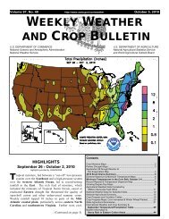
<strong>Drought</strong>s also differ in terms <strong>of</strong> their spatial characteristics. <strong>Drought</strong>s are regional in nature and<br />
may affect millions <strong>of</strong> square kilometers (Figure 1). Because <strong>of</strong> drought’s long duration, its<br />
epicenter shifts from season to season and from year to year. <strong>Drought</strong> monitoring systems must<br />
rely on multiple indicators to adequately identify areas <strong>of</strong> maximum severity and be able to<br />
evaluate how changes in the spatial dimension <strong>of</strong> drought alter current and future impacts and the<br />
activation and termination <strong>of</strong> mitigation actions and emergency programs.<br />
Figure 1. Percent area <strong>of</strong> the United States in severe and extreme drought, January 1895-May 2010.<br />
<strong>Drought</strong> Risk and Vulnerability Assessment<br />
Many people consider drought to be largely a natural or physical event. In reality, drought, like<br />
other natural hazards, has both a natural and a social component (Wilhite 2009). The risk<br />
associated with drought for any region is a product <strong>of</strong> both the region’s exposure to the event and<br />
the vulnerability <strong>of</strong> society to the event. Exposure to drought varies regionally and there is little, if<br />
anything, we can do to reduce the recurrence, frequency, or incidence <strong>of</strong> the event. It is <strong>of</strong> critical<br />
importance that countries develop a comprehensive understanding <strong>of</strong> the climatology <strong>of</strong> drought<br />
and how the frequency, severity, and duration <strong>of</strong> these extreme climatic events vary spatially.<br />
15
Understanding the nature <strong>of</strong> the hazard helps identify those regions most at risk to drought<br />
because <strong>of</strong> varying degrees <strong>of</strong> exposure.<br />
In order to have a more complete picture <strong>of</strong> drought risk, however, we must also understand our<br />
vulnerability, which is the product <strong>of</strong> social factors. Population is not only increasing but also<br />
shifting from humid (i.e., water surplus) to more arid (i.e., water deficit) climates and from rural to<br />
urban settings for many locations. As population increases, so does pressure on natural resources.<br />
People are also forced to reside in climatically marginal, more drought-prone areas. Urbanization<br />
is placing more pressure on limited water supplies and the capacity <strong>of</strong> water supply systems to<br />
deliver that water to users, especially during periods <strong>of</strong> peak demand. An increasingly urbanized<br />
population is also increasing conflict between agricultural and urban water users, a trend that will<br />
only be exacerbated in the future. Increasingly sophisticated technology decreases our<br />
vulnerability to drought in some instances while increasing it in others. Greater awareness <strong>of</strong> our<br />
environment and the need to preserve and restore environmental quality is placing greater<br />
pressure on all <strong>of</strong> us to be better stewards <strong>of</strong> natural and biological resources. Environmental<br />
degradation (i.e., desertification) is reducing the productivity <strong>of</strong> some landscapes and increasing<br />
vulnerability to drought events. All <strong>of</strong> these factors emphasize that our vulnerability to drought is<br />
dynamic and must be reevaluated periodically so that we understand how these changes will affect<br />
us and who and what are most at risk for future drought events. We should expect the impacts <strong>of</strong><br />
drought in the future to be different, more complex, and more significant for some economic<br />
sectors, population groups, and regions. The world’s dryland areas are most at risk to changes in<br />
exposure and the pressures <strong>of</strong> increasing populations. Improving drought management implies an<br />
attempt to use natural resources in a more sustainable manner. This will require a partnership<br />
between individuals and government.<br />
<strong>Drought</strong>s have occurred in the past and they will continue to occur in the future since they are a<br />
normal part <strong>of</strong> climate. The impacts associated with drought may increase because <strong>of</strong> an<br />
increased exposure to the event, increased societal vulnerability, or a combination <strong>of</strong> the two. For<br />
this reason, it is imperative that countries assess their exposure to drought (i.e., historical analysis<br />
<strong>of</strong> drought and its characteristics) and conduct a vulnerability assessment (i.e., create a<br />
vulnerability pr<strong>of</strong>ile) to determine who and what is at risk and why. It is also important to critically<br />
assess how exposure to drought may change in the future because <strong>of</strong> changes in climate<br />
variability or climate state and how these changes may affect future vulnerability and adaptation<br />
strategies.<br />
Scientific investigations <strong>of</strong> climate change resulting from an increased concentration <strong>of</strong> greenhouse<br />
gases in the atmosphere suggest that the incidence and severity <strong>of</strong> meteorological drought may<br />
increase for some regions in the future (Pachauri and Reisinger 2007). In recent years, numerous<br />
countries have experienced an increased incidence <strong>of</strong> meteorological drought, but it is unknown at<br />
present whether this increase is the result <strong>of</strong> climate change or a part <strong>of</strong> normal climate variability.<br />
Regardless, this increased frequency <strong>of</strong> drought has resulted in significant consequences and<br />
greater awareness <strong>of</strong> the need to plan for drought events. Developing countries have been<br />
particularly affected because they <strong>of</strong>ten lack the institutional capacity to deal effectively with<br />
extended drought episodes.<br />
<strong>Drought</strong> Monitoring and Early Warning<br />
Effective drought early warning systems (DEWS) are an integral part <strong>of</strong> efforts worldwide to<br />
improve drought preparedness. Timely and reliable data and information must be the cornerstone<br />
<strong>of</strong> effective drought policies and plans. Monitoring drought presents some unique challenges<br />
because <strong>of</strong> drought’s distinctive characteristics.<br />
An expert group meeting on early warning systems for drought preparedness, sponsored by the<br />
World Meteorological Organization (WMO) and others, recently examined the status, shortcomings,<br />
and needs <strong>of</strong> DEWS, and made recommendations on how these systems can help in achieving a<br />
greater level <strong>of</strong> drought preparedness (Wilhite et al. 2000b). This meeting was organized as part<br />
<strong>of</strong> WMO’s contribution to the UNCCD. The proceedings <strong>of</strong> this meeting documented recent efforts<br />
16
in DEWS in countries such as Brazil, China, Hungary, India, Nigeria, South Africa, and the United<br />
States, but also noted the activities <strong>of</strong> regional drought monitoring centers in eastern and southern<br />
Africa and efforts in West Asia and North Africa. Shortcomings <strong>of</strong> current DEWS were noted in the<br />
following areas:<br />
• data networks—inadequate density and data quality <strong>of</strong> meteorological and hydrological<br />
networks and lack <strong>of</strong> data networks on all major climate and water supply parameters;<br />
• data sharing—inadequate data sharing between government agencies and the high cost <strong>of</strong><br />
data limit the application <strong>of</strong> data in drought preparedness, mitigation, and response;<br />
• early warning system products—data and information products are <strong>of</strong>ten not user friendly<br />
and users are <strong>of</strong>ten not trained in the application <strong>of</strong> this information to decision making;<br />
• drought forecasts—unreliable seasonal forecasts and the lack <strong>of</strong> specificity <strong>of</strong> information<br />
provided by forecasts limit the use <strong>of</strong> this information by farmers and others;<br />
• drought monitoring tools—inadequate indices for detecting the early onset and end <strong>of</strong><br />
drought, although the Standardized Precipitation Index (SPI) was cited as an important new<br />
monitoring tool to detect the early emergence <strong>of</strong> drought;<br />
• integrated drought/climate monitoring—drought monitoring systems should be integrated<br />
and based on multiple indicators to fully understand drought magnitude, spatial extent, and<br />
impacts;<br />
• drought impact assessment methodology—lack <strong>of</strong> impact assessment methodology<br />
hinders impact estimates and the activation <strong>of</strong> mitigation and response programs;<br />
• delivery systems—data and information on emerging drought conditions, seasonal<br />
forecasts, and other products are <strong>of</strong>ten not delivered to users in a timely manner;<br />
• global drought early warning system—no historical drought database exists and there is no<br />
global drought assessment product that is based on one or two key indicators, which could<br />
be helpful to international organizations, NGOs, and others.<br />
Participants <strong>of</strong> the expert group meeting on DEWS made several recommendations. Those<br />
recommendations that pertained directly to early warning systems were that these systems should<br />
be considered an integral part <strong>of</strong> drought preparedness and mitigation plans and that priority<br />
should be given to improving existing observation networks and establishing new meteorological,<br />
agricultural, and hydrological networks.<br />
Effective drought monitoring requires the integration <strong>of</strong> a variety <strong>of</strong> indices and indicators. <strong>Indices</strong><br />
commonly used to monitor drought and rainfall conditions include the Standardized Precipitation<br />
Index, deciles, percent <strong>of</strong> normal rainfall/precipitation, the Palmer <strong>Drought</strong> Severity Index, the<br />
Surface Water Supply Index, and the Vegetation Condition Index, among others (see, for example,<br />
the U.S. <strong>Drought</strong> Monitor [http://drought.unl.edu/dm/]). Other indicators <strong>of</strong> drought <strong>of</strong>ten used to<br />
monitor conditions include soil moisture, snowpack, streamflow, groundwater levels, reservoir and<br />
lake levels, vegetation health, and short-, medium-, and long-range forecasts. Remote sensing<br />
<strong>of</strong>fers new and exciting opportunities to monitor drought conditions because <strong>of</strong> higher resolution.<br />
These techniques are especially advantageous in regions lacking adequate weather station<br />
networks.<br />
Considering the complexity <strong>of</strong> drought and the many indices and indicators necessary to assess its<br />
severity and likely impacts, the most successful approach to date (drought.unl.edu/dm) is the U.S.<br />
<strong>Drought</strong> Monitor (Figure 2). This map is produced weekly through a collaborative partnership<br />
between the U.S. <strong>Department</strong> <strong>of</strong> <strong>Agriculture</strong>, the National Oceanic and Atmospheric Administration,<br />
and the National <strong>Drought</strong> Mitigation Center at the University <strong>of</strong> Nebraska. It incorporates multiple<br />
indices and indicators <strong>of</strong> drought, including impacts, into the assessment process. Although many<br />
countries do not have the range <strong>of</strong> data available to replicate this process fully, any approach that<br />
incorporates information beyond precipitation and, perhaps, temperature data is going to provide a<br />
more accurate picture <strong>of</strong> drought severity.<br />
17
Figure 2. U.S. <strong>Drought</strong> Monitor for July 28, 2009.<br />
<strong>Drought</strong> Policy and Preparedness<br />
Article 10 <strong>of</strong> the U.N. Convention to Combat Desertification (UNCCD) states that national action<br />
programs should be established to “identify the factors contributing to desertification and practical<br />
measures necessary to combat desertification and mitigate the effects <strong>of</strong> drought” (UNCCD 1999).<br />
In the past 10 years there has been considerable recognition by governments <strong>of</strong> the need to<br />
develop drought preparedness plans and policies to reduce the impacts <strong>of</strong> drought. Unfortunately,<br />
progress in drought preparedness during the last decade has been slow because most nations<br />
lack the institutional capacity and human and financial resources necessary to develop<br />
comprehensive drought plans and policies. Recent commitments by governments and international<br />
organizations and new drought monitoring technologies and planning and mitigation<br />
methodologies are cause for optimism. The challenge is the implementation <strong>of</strong> these new policies,<br />
methodologies, and technologies.<br />
One <strong>of</strong> the trends associated with recent drought events has been the growing complexity <strong>of</strong><br />
drought impacts. Past drought impacts have been linked most closely to the agricultural sector,<br />
reducing the capacity <strong>of</strong> many nations to be food secure. In both developing and developed<br />
countries the impacts <strong>of</strong> drought are <strong>of</strong>ten an indicator <strong>of</strong> non-sustainable land and water<br />
management practices, and drought assistance or relief provided by governments and donors<br />
<strong>of</strong>ten encourages land managers and others to continue these practices. It is precisely these<br />
existing resource management practices that have <strong>of</strong>ten increased societal vulnerability to drought<br />
(i.e., exacerbated drought impacts). This <strong>of</strong>ten results in decreased resilience <strong>of</strong> individuals and<br />
communities and an increased dependence on government. One <strong>of</strong> the principal goals <strong>of</strong> drought<br />
policies and preparedness plans is to move societies away from the traditional approach <strong>of</strong> crisis<br />
management, which is reactive in nature, to a more pro-active, risk management approach. The<br />
goal <strong>of</strong> risk management is to promote the adoption <strong>of</strong> preventative or risk-reducing measures and<br />
strategies that will mitigate the impacts <strong>of</strong> future drought events, thus reducing societal vulnerability.<br />
18
This paradigm shift emphasizes preparedness, mitigation, and improved early warning systems<br />
(EWS) over emergency response and assistance measures.<br />
<strong>Drought</strong>-prone nations should develop national drought policies and preparedness plans that place<br />
emphasis on risk management rather than the traditional approach <strong>of</strong> crisis management, where<br />
the emphasis is on reactive emergency response measures (Botterill and Wilhite 2005). Crisis<br />
management decreases self-reliance and increases dependence on government and donors. This<br />
approach has been ineffective because response is untimely (i.e., post-impact), poorly coordinated<br />
within and between levels <strong>of</strong> government and with donor organizations and NGOs, and poorly<br />
targeted to drought-stricken groups or areas. Many governments and others now understand the<br />
fallacy <strong>of</strong> crisis management and are striving to learn how to employ proper risk management<br />
techniques to reduce societal vulnerability to drought and therefore lessen the impacts associated<br />
with future drought events.<br />
Developing vulnerability pr<strong>of</strong>iles for regions, communities, population groups, and others will<br />
provide critical information on who and what is at risk and why. This information, when integrated<br />
into the planning process, can enhance the outcome <strong>of</strong> the process by identifying and prioritizing<br />
specific areas where progress can be made in risk management.<br />
In the past decade or so, drought policy and preparedness plans have received increasing<br />
attention from governments, international and regional organizations, and NGOs. Simply stated, a<br />
national drought policy should establish a clear set <strong>of</strong> principles or operating guidelines to govern<br />
the management <strong>of</strong> drought and its impacts (Wilhite 2000a). The policy should be consistent and<br />
equitable for all regions, population groups, and economic sectors and consistent with the goals <strong>of</strong><br />
sustainable development. The overriding principle <strong>of</strong> drought policy should be an emphasis on risk<br />
management through the application <strong>of</strong> preparedness and mitigation measures. Preparedness<br />
refers to pre-disaster activities designed to increase the level <strong>of</strong> readiness or improve operational<br />
and institutional capabilities for responding to a drought episode. Mitigation actions, programs, or<br />
policies are implemented during and in advance <strong>of</strong> drought to reduce the degree <strong>of</strong> risk to human<br />
life, property, and productive capacity. Emergency response will always be a part <strong>of</strong> drought<br />
management because it is unlikely that government and others can anticipate, avoid, or reduce all<br />
potential impacts through mitigation programs. A future drought event may also exceed the<br />
“drought <strong>of</strong> record” and the capacity <strong>of</strong> a region to respond. However, emergency response<br />
should be used sparingly and only if it is consistent with longer-term drought policy goals and<br />
objectives.<br />
A national drought policy should be directed toward reducing risk by developing better awareness<br />
and understanding <strong>of</strong> the drought hazard and the underlying causes <strong>of</strong> societal vulnerability. The<br />
principles <strong>of</strong> risk management can be promoted by encouraging the improvement and application<br />
<strong>of</strong> seasonal and shorter-term forecasts, developing integrated monitoring and drought EWS and<br />
associated information delivery systems, developing preparedness plans at various levels <strong>of</strong><br />
government, adopting mitigation actions and programs, and creating a safety net <strong>of</strong> emergency<br />
response programs that ensure timely and targeted relief.<br />
One thing is certain: continuing to address drought impacts in a reactive, crisis management mode<br />
will do little to reduce the impacts <strong>of</strong> these events in the future. If government continues to “bail<br />
out” those people most affected by drought, they will have no incentive to adopt methods that will<br />
improve protection <strong>of</strong> the natural resource base. Should society subsidize poor land managers or<br />
reward good land managers? Risk management is aimed at the latter; crisis management, the<br />
former. It is precisely these existing resource management practices that have <strong>of</strong>ten increased<br />
societal vulnerability to drought (i.e., exacerbated drought impacts). Many governments and<br />
others now understand the fallacy <strong>of</strong> crisis management and are striving to learn how to employ<br />
proper risk management techniques to reduce societal vulnerability to drought and therefore<br />
lessen the impacts associated with future drought events.<br />
19
Summary<br />
<strong>Drought</strong> is a creeping phenomenon with no universal definition. Definitions <strong>of</strong> drought must be<br />
region and application or impact specific. Many indices and indicators are available to assist in the<br />
quantitative assessment <strong>of</strong> drought severity, and these should be evaluated carefully for their<br />
application to each region or location and sector. To best characterize drought it is critically<br />
important to use a combination <strong>of</strong> indices and indicators since no single one can capture the full<br />
severity <strong>of</strong> a particular drought event. This is an especially difficult assignment for agricultural and<br />
hydrological drought.<br />
Data sources are varied between countries, and the development <strong>of</strong> an effective drought early<br />
warning and delivery system requires interagency cooperation to assess drought severity, impacts,<br />
and the implementation <strong>of</strong> appropriate mitigation strategies. The development <strong>of</strong> systems to<br />
deliver that information to decision makers at all levels requires their active participation in the<br />
development <strong>of</strong> decision support tools from the earliest stages <strong>of</strong> that process.<br />
<strong>Drought</strong> risk is best defined as a combination <strong>of</strong> a location’s exposure to drought and its<br />
vulnerability to drought. Exposure to drought is characterized through an analysis <strong>of</strong> the historical<br />
climatology <strong>of</strong> a region, including an analysis <strong>of</strong> trends or changes in climate state and/or its<br />
variability. <strong>Drought</strong> impacts are a key indicator <strong>of</strong> vulnerability. Therefore, conducting a<br />
vulnerability assessment involves an analysis <strong>of</strong> the historical impacts associated with previous<br />
drought episodes. Since societies are constantly changing, vulnerabilities are also likely to change<br />
due to increasing population, land degradation, urbanization, technology, and many other factors.<br />
Each occurrence <strong>of</strong> drought for a particular region is layered upon a society with differing<br />
vulnerabilities.<br />
Early warning systems are the foundation <strong>of</strong> effective drought mitigation and preparedness plans.<br />
The goal <strong>of</strong> our meeting on the selection <strong>of</strong> appropriate drought indices or indicators to<br />
characterize agricultural drought was to reach consensus on a single index to accomplish this task.<br />
That is a formidable task given the complexities <strong>of</strong> agricultural drought and the variable institutional<br />
capacity <strong>of</strong> drought-prone nations. At best, we should strive to identify a series <strong>of</strong> alternative<br />
approaches to characterize agricultural drought in various settings depending on available data<br />
and local capabilities. As a part <strong>of</strong> this approach, we should continue to work toward implementing<br />
a composite approach (i.e., incorporate multiple indices and indicators) to characterizing<br />
agricultural drought.<br />
References<br />
Alley, W.M. 1984. The Palmer <strong>Drought</strong> Severity Index: Limitations and assumptions. Journal <strong>of</strong><br />
Climate and Applied Meteorology 23:1,100-1,109.<br />
Botterill, L. Courtenay and D.A. Wilhite. 2005. From Disaster Response to Risk Management:<br />
Australia’s National <strong>Drought</strong> Policy. Springer, Dordrecht, The Netherlands.<br />
Coughlan, M.J. 1987. Monitoring drought in Australia. Pages 131-144 in Planning for <strong>Drought</strong>:<br />
Toward a Reduction <strong>of</strong> Societal Vulnerability (D. A. Wilhite and W. E. Easterling, eds.).<br />
Westview Press, Boulder, Colorado.<br />
Gibbs, W.J. and J.V. Maher. 1967. Rainfall deciles as drought indicators. Bureau <strong>of</strong> Meteorology<br />
Bulletin No. 48. Melbourne, Australia.<br />
Guttman, N.B. 1998. Comparing the Palmer <strong>Drought</strong> Index and the Standardized Precipitation<br />
Index. Journal <strong>of</strong> the American Water Resources Association 34 (1):113-21.<br />
Lee, D.M. 1979. Australian drought watch system. Pages 173-187 in Botswana <strong>Drought</strong><br />
Symposium (M.T. Hinchey, ed.). Botswana Society, Gaborone, Botswana.<br />
McKee, T.B., N.J. Doesken, and J. Kleist. 1993. The relationship <strong>of</strong> drought frequency and<br />
duration to time scales. Eighth Conference on Applied Climatology. American<br />
Meteorological Society, Boston.<br />
McKee, T.B., N.J. Doesken, and J. Kleist. 1995. <strong>Drought</strong> monitoring with multiple time scales.<br />
Ninth Conference on Applied Climatology. American Meteorological Society, Boston.<br />
20
Pachauri, R.K. and A. Reisinger (eds.). 2007. Climate Change 2007: Synthesis Report.<br />
Intergovernmental Panel on Climate Change. Geneva, Switzerland.<br />
Palmer, W.C. 1965. Meteorological drought. Research Paper No. 45. U.S. Weather Bureau,<br />
Washington, D.C.<br />
Palmer, W. C. 1968. Keeping track <strong>of</strong> crop moisture conditions, nationwide: The new crop<br />
moisture index. Weatherwise 21(4):156-61.<br />
UNCCD. 1999. United Nations Convention to Combat Desertification (text with annexes). Bonn,<br />
Germany.<br />
Wilhite, D.A. and M.H. Glantz. 1985. Understanding the drought phenomenon: The role <strong>of</strong><br />
definitions. Water International 10:111-120.<br />
Wilhite, D.A. (ed.). 2000. <strong>Drought</strong>: A Global Assessment (2 volumes, 51 chapters, 700 pages).<br />
Hazards and Disasters: A Series <strong>of</strong> Definitive Major Works (7-volume series), edited by A.Z.<br />
Keller. Routledge Publishers, London, U.K.<br />
Wilhite, D.A., M.J. Hayes, C. Knutson, and K.H. Smith. 2000a. Planning for drought: Moving from<br />
crisis to risk management. Journal <strong>of</strong> the American Water Resources Association 36:697-<br />
710.<br />
Wilhite, D.A., M.K.V. Sivakumar, and D.A. Wood (eds.). 2000b. Early Warning Systems for<br />
<strong>Drought</strong> Preparedness and Management (Proceedings <strong>of</strong> an Experts Meeting). World<br />
Meteorological Organization, Geneva, Switzerland.<br />
Wilhite, D.A. and M. Buchanan-Smith. 2005. <strong>Drought</strong> as hazard: Understanding the natural and<br />
social context. Chapter 1 in <strong>Drought</strong> and Water Crises: Science, Technology, and<br />
Management Issues (D.A. Wilhite, ed.). CRC Press, Boca Raton, Florida.<br />
Wilhite, D.A. 2009. The role <strong>of</strong> monitoring as a component <strong>of</strong> preparedness planning: Delivery <strong>of</strong><br />
information and decision support tools. Chapter 1 in Coping with <strong>Drought</strong> Risk and<br />
<strong>Agriculture</strong> and Water Supply Systems: <strong>Drought</strong> Policy and Policy Development in the<br />
Mediterranean (A. Iglesias, L. Garrote, A. Cancelliere, F. Cubillo, and D.A. Wilhite, eds.).<br />
Springer, Dordrecht, The Netherlands.<br />
21
<strong>Agricultural</strong> <strong>Drought</strong>—WMO Perspectives<br />
Mannava V.K. Sivakumar<br />
World Meteorological Organization, Switzerland<br />
Abstract<br />
The increasing frequency and magnitude <strong>of</strong> droughts in recent decades and the mounting losses<br />
from extended droughts in the agricultural sector emphasize the need for assigning an urgent<br />
priority to addressing the issue <strong>of</strong> agricultural droughts. As the United Nations specialized agency<br />
with responsibility for meteorology and operational hydrology, WMO, since its inception, has been<br />
addressing the issue <strong>of</strong> droughts. In this respect, WMO promotes systematic observation,<br />
collection, analysis, and exchange <strong>of</strong> meteorological, climatological, and hydrological data and<br />
information; drought planning preparedness and management; research into the causes and<br />
effects <strong>of</strong> climate variations and long-term climate predictions with a view to providing early<br />
warning; capacity building; and the transfer <strong>of</strong> knowledge and technology.<br />
The fight against drought receives a high priority in the Long-term Plan <strong>of</strong> WMO, particularly under<br />
the <strong>Agricultural</strong> Meteorology Programme, Hydrology and Water Resources Programme, and<br />
Technical Cooperation Programme. Within the context <strong>of</strong> this Plan, WMO continues to encourage<br />
the greater involvement <strong>of</strong> the national Meteorological and Hydrological Services (NMHSs) and<br />
regional and subregional meteorological and hydrological centers in addressing the issues <strong>of</strong><br />
drought.<br />
This paper presents a short description <strong>of</strong> the perspectives <strong>of</strong> the World Meteorological<br />
Organization (WMO) on drought in general and agricultural drought in particular. This is followed<br />
by a short narrative on WMO’s activities in the area <strong>of</strong> drought. The Commission for <strong>Agricultural</strong><br />
Meteorology (CAgM) <strong>of</strong> WMO since 1967 has appointed a number <strong>of</strong> working groups and<br />
rapporteurs with specific terms <strong>of</strong> reference. These have mainly addressed several applications,<br />
including drought monitoring, forecasting, and control; meteorological aspects <strong>of</strong> drought<br />
processes; operational use <strong>of</strong> agrometeorology; measures to alleviate the effects <strong>of</strong> droughts;<br />
assessment <strong>of</strong> the economic impacts; and capacity-building activities. A number <strong>of</strong> different<br />
indices have been used to describe agricultural droughts, and some examples are presented.<br />
The role played by NMHSs in drought monitoring, risk assessment, and early warning is described<br />
with examples from China, South Africa, and Portugal. WMO has also been placing considerable<br />
importance on organizing capacity-building activities in the area <strong>of</strong> drought preparedness and<br />
management, especially in the developing countries, and a list <strong>of</strong> activities carried out since 1990<br />
is presented. WMO’s support in strengthening the capabilities <strong>of</strong> regional institutions with droughtrelated<br />
programs and in promoting collaboration with other institutions in drought- and<br />
desertification-prone regions is described.<br />
Introduction<br />
<strong>Drought</strong> is a normal, recurrent climatic feature that occurs in virtually every climatic zone around<br />
the world, causing billions <strong>of</strong> dollars in loss annually for the farming community. <strong>Drought</strong> ranks first<br />
among all natural hazards according to Bryant (1991), who ranked natural hazard events based on<br />
various characteristics, such as severity, duration, spatial extent, loss <strong>of</strong> life, economic loss, social<br />
effect, and long-term impact. This is because, compared to other natural hazards like flood and<br />
hurricanes that develop quickly and last for a short time, drought is a creeping phenomenon that<br />
accumulates over a period <strong>of</strong> time across a vast area, and the effect lingers for years even after<br />
the end <strong>of</strong> drought (Tannehill 1947). Hence, the loss <strong>of</strong> life, economic impact, and effects on<br />
society are spread over a long period <strong>of</strong> time, which makes drought the worst among all natural<br />
hazards. For example, the Murray-Darling River Basin in Australia was subjected to periods <strong>of</strong><br />
protracted drought with two decade-long droughts in the last century. Since 2001 it has been<br />
experiencing the worst drought in recorded history. System inflows in the three years ending<br />
22
October 2008 were almost half the previous three-year minimum and less than a quarter <strong>of</strong> the<br />
long-term average. In 2010, the worst drought in six decades in southwest China has plunged<br />
more than 2 million people back into poverty. A severe drought has swept the southwestern region,<br />
including Yunnan, Sichuan, and Guizhou provinces; Guangxi Zhuang autonomous region; and<br />
Chongqing municipality.<br />
Because drought affects so many economic and social sectors, scores <strong>of</strong> definitions have been<br />
developed by a variety <strong>of</strong> disciplines. Wilhite and Glantz (1985) analyzed more than 150 such<br />
definitions <strong>of</strong> drought and then broadly grouped those definitions under four categories:<br />
meteorological, agricultural, hydrological, and socio-economic drought.<br />
Losses from extended droughts in the agricultural sector can <strong>of</strong>ten amount to hundreds <strong>of</strong> millions<br />
<strong>of</strong> dollars. Direct losses result from reduced crop yields, diminished pasture growth, and mortality<br />
<strong>of</strong> livestock while indirect losses include lost opportunities in agriculture and livestock sectors and<br />
losses to abandonment <strong>of</strong> land and changes in land use following droughts. According to the U.S.<br />
Federal Emergency Management Agency (FEMA), the United States loses $6-8 billion annually on<br />
average because <strong>of</strong> drought (FEMA 1995). During the 1998 drought, the state <strong>of</strong> Texas alone lost<br />
a staggering $5.8 billion (Chenault and Parsons 1998), which is about 39% <strong>of</strong> the $15 billion<br />
annual agriculture revenue <strong>of</strong> the state (Sharp 1996). The aggregate impact <strong>of</strong> drought can be<br />
quite negative on the economies <strong>of</strong> developing countries, in particular. For example, GDP fell by 8-<br />
9% in Zimbabwe and Zambia in 1992 and 4-6% in Nigeria and Niger in 1984.<br />
This paper presents a short description <strong>of</strong> the perspectives <strong>of</strong> the World Meteorological<br />
Organization (WMO) on drought in general and agricultural drought in particular. This is followed<br />
by a short narrative on WMO’s activities in the area <strong>of</strong> drought.<br />
WMO’s Focus on <strong>Drought</strong><br />
As the United Nations specialized agency with responsibility for meteorology and operational<br />
hydrology, WMO, since its inception, has been addressing the issue <strong>of</strong> droughts. In this respect,<br />
WMO promotes systematic observation, collection, analysis, and exchange <strong>of</strong> meteorological,<br />
climatological, and hydrological data and information; drought planning preparedness and<br />
management; research into the causes and effects <strong>of</strong> climate variations and long-term climate<br />
predictions with a view to providing early warning; capacity building; and the transfer <strong>of</strong> knowledge<br />
and technology.<br />
The fight against drought receives a high priority in the Long-term Plan <strong>of</strong> WMO, particularly under<br />
the <strong>Agricultural</strong> Meteorology Programme, Hydrology and Water Resources Programme, and<br />
Technical Cooperation Programme. Within the context <strong>of</strong> this Plan, WMO continues to encourage<br />
the greater involvement <strong>of</strong> the national Meteorological and Hydrological Services (NMHSs) and<br />
regional and subregional meteorological and hydrological centers in addressing the issues <strong>of</strong><br />
drought.<br />
The Commission for <strong>Agricultural</strong> Meteorology (CAgM) <strong>of</strong> WMO has been very active in addressing<br />
the issue <strong>of</strong> agricultural drought and made recommendations regarding the role <strong>of</strong><br />
agrometeorology in helping to solve drought problems in drought-stricken areas, particularly in<br />
Africa. The Commission appointed a number <strong>of</strong> working groups and rapporteurs with specific<br />
terms <strong>of</strong> reference. Based on the activities <strong>of</strong> these working groups and rapporteurs, a number <strong>of</strong><br />
reports were published and distributed by WMO.<br />
Working Groups on <strong>Drought</strong> Appointed by CAgM (1967-2010)<br />
Following are the working groups on drought appointed by CAgM at its sessions since 1967:<br />
a) Fourth Session <strong>of</strong> CAgM (CAgM-IV) (Manila, Philippines, 1967) – Working Group on<br />
Assessment <strong>of</strong> <strong>Drought</strong><br />
b) CAgM-V (Geneva, Switzerland, 1971) – Working Group on the Meteorological Factors<br />
Concerning Certain Aspects <strong>of</strong> Soil Deterioration and Erosion<br />
23
c) CAgM-VI (Washington, <strong>US</strong>A, 1974) – Rapporteur on the Frequency and Impact <strong>of</strong> Water<br />
Deficiencies for Selected Plant-Soil Systems (Resolution 2) – <strong>Drought</strong> and <strong>Agriculture</strong><br />
d) CAgM-VII (S<strong>of</strong>ia, Bulgaria, 1979) – Working Group on the Agrometeorological Aspects <strong>of</strong><br />
Land Management in the Arid and Semi-Arid Areas with special reference to Desertification<br />
Problems; Rapporteur on <strong>Drought</strong> Probability Maps<br />
e) CAgM-VIII (Geneva, Switzerland, 1983) – Working Group on Meteorological Aspects <strong>of</strong><br />
<strong>Agriculture</strong> in <strong>Drought</strong>-Prone and Semi-Arid Areas; Rapporteur on <strong>Drought</strong> Probability<br />
Maps<br />
f) CAgM-IX (Madrid, Spain, 1986) – Working Group on Monitoring, Assessment and Combat<br />
<strong>of</strong> <strong>Drought</strong> and Desertification<br />
g) CAgM-X (Florence, Italy, 1991) – Working Group on Extreme Meteorological Events<br />
h) CAgM-XI (Havana, Cuba, 1995) – Working Group on Desertification and <strong>Drought</strong><br />
i) CAgM-XII (Accra, Ghana, 1999) – Working Group on the Impacts <strong>of</strong> Desertification and <strong>of</strong><br />
<strong>Drought</strong> and other Extreme Meteorological Events<br />
j) CAgM-XIII (Ljubljana, Slovenia, 2002) – Expert Team on Reduction <strong>of</strong> the Impact <strong>of</strong> Natural<br />
Disasters and Mitigation <strong>of</strong> Extreme Events in <strong>Agriculture</strong>, Rangelands, Forestry and<br />
Fisheries<br />
k) CAgM-XIV (New Delhi, India, 2006) - Expert Team on <strong>Drought</strong> and Extreme Temperatures:<br />
Preparedness and Management for Sustainable <strong>Agriculture</strong>, Rangelands, Forestry, and<br />
Fisheries<br />
l) CAgM-XV (Belo Horizonte, Brazil, 2010) – Expert Team on Weather and Climate Extremes<br />
and Impacts and Preparedness Strategies in <strong>Agriculture</strong>, Rangelands, Forestry, and<br />
Fisheries<br />
WMO Publications on <strong>Drought</strong> and Agrometeorological Applications Addressed<br />
Following are important titles on drought produced by CAgM since 1963:<br />
a) <strong>Drought</strong> and <strong>Agriculture</strong> (WMO 1975)<br />
b) <strong>Drought</strong> Probability Maps (WMO 1987)<br />
c) <strong>Drought</strong> and Desertification in Asia (WMO 1988)<br />
d) Climate Applications Referral System – Desertification (WMO 1989)<br />
e) Report on <strong>Drought</strong> and Desertification (WMO 1992)<br />
f) Monitoring, Assessment, and Combat <strong>of</strong> <strong>Drought</strong> and Desertification (WMO 1992)<br />
g) <strong>Drought</strong> Preparedness and Management for Western African Countries (WMO 1995)<br />
h) WMO/UNEP Publication on Interactions <strong>of</strong> Desertification and Climate (Williams and<br />
Balling 1996)<br />
i) Climate, <strong>Drought</strong> and Desertification (WMO 1997)<br />
j) La prévention et la gestion des situations de sécheresse dans les pays du Maghreb (WMO<br />
1998)<br />
k) Early Warning Systems for <strong>Drought</strong> and Desertification: Role <strong>of</strong> National Meteorological<br />
and Hydrological Services (WMO 1999)<br />
l) Early Warning Systems for <strong>Drought</strong> Preparedness and <strong>Drought</strong> Management (WMO 2000)<br />
m) Coping with <strong>Drought</strong> in Sub-Saharan Africa: Better Use <strong>of</strong> Climate Information (WMO 2000)<br />
n) <strong>Drought</strong> Monitoring and Early Warning: Concepts, Progress, and Future Challenges (WMO<br />
2006)<br />
<strong>Drought</strong> Applications Addressed by WMO<br />
The activities <strong>of</strong> the different working groups and rapporteurs on drought appointed by CAgM, and<br />
the publications on drought produced over the years, mainly addressed the following applications:<br />
• <strong>Drought</strong> monitoring, forecasting, and control<br />
• Meteorological aspects <strong>of</strong> drought processes<br />
• Operational use <strong>of</strong> agrometeorology<br />
• Measures to alleviate the effects <strong>of</strong> droughts<br />
• Assessment <strong>of</strong> economic impacts<br />
• Capacity-building activities<br />
24
WMO’s Perspectives on <strong>Drought</strong><br />
Given the extensive number <strong>of</strong> activities undertaken, it will be difficult to provide an exhaustive<br />
description <strong>of</strong> WMO’s perspectives on droughts in this short paper. Hence, a short description <strong>of</strong><br />
different perspectives is provided below, using the material from the different publications listed<br />
above.<br />
Understanding <strong>of</strong> <strong>Drought</strong>s and <strong>Drought</strong> Definitions<br />
WMO’s early efforts placed emphasis on many meteorological facets <strong>of</strong> drought, including its<br />
definition and early recognition; its effect on plants, animals, and diseases; and methods <strong>of</strong><br />
surviving under its influence. Clarifications were provided on the distinction between drought and<br />
aridity; the linkage between drought and water balance (soil water, precipitation, dew and fog, and<br />
surface run<strong>of</strong>f); fire hazards; drought, ecological imbalance, and soil erosion; the space and time<br />
characteristics <strong>of</strong> droughts; causes <strong>of</strong> droughts; and forecasting <strong>of</strong> droughts (WMO 1975). Some<br />
detailed studies <strong>of</strong> past droughts suggested that changes in the surface albedo, existence <strong>of</strong> a<br />
deep dust layer in the atmosphere, changes in sea surface temperatures, and an increase <strong>of</strong><br />
carbon dioxide may lead to changes in the general circulation features, which may cause drought<br />
(WMO 1987).<br />
<strong>Drought</strong> definitions used over time vary from region to region and according to the purpose for<br />
which they are defined. A general survey <strong>of</strong> drought definitions has indicated that they can be<br />
classified according to the criteria used. A classification <strong>of</strong> drought definitions was given (WMO<br />
1975) under each <strong>of</strong> the following subheadings:<br />
a) Rainfall<br />
b) Rainfall with mean temperature<br />
c) Soil water and crop parameters<br />
d) Climatic indices and estimates <strong>of</strong> evapotranspiration<br />
e) General definitions and statements<br />
As an example, looking more closely into definitions based solely on rainfall, it was shown that a<br />
number <strong>of</strong> these refer to short period “droughts” or “dry spells” (WMO 1975).<br />
• Less than 2.5 mm in 48 hours<br />
• Rainfall half <strong>of</strong> normal or less for a week<br />
• 10 days with rainfall not exceeding 5 mm<br />
• 15 days with no rain<br />
• 15 consecutive days, none with 0.25 mm<br />
• 15 consecutive days, none with 1 mm<br />
• 21 days or more with rainfall less than 30% <strong>of</strong> normal<br />
• 21 days with precipitation less than one-third <strong>of</strong> normal<br />
These appeared to be geared mainly to climatic experience in the British Isles or perhaps the<br />
northeastern United States, where rainfall is received at fairly frequent intervals and crop and<br />
animal husbandry and water-storage operations are not geared to the long spells <strong>of</strong> rainless<br />
weather that are seasonally normal in the semiarid regions (WMO 1975).<br />
<strong>Agricultural</strong> <strong>Drought</strong> and <strong>Drought</strong> Index<br />
<strong>Agriculture</strong> is <strong>of</strong>ten the first sector to be impacted by drought because access to water resources<br />
and soil moisture reserves determine crop productivity. <strong>Drought</strong> in the agricultural sense does not<br />
begin with the cessation <strong>of</strong> rain, but rather when available stored water will support actual<br />
evapotranspiration at only a small fraction <strong>of</strong> the potential evapotranspiration rate (WMO 1992).<br />
The rate <strong>of</strong> transpiration by a crop depends largely upon the availability <strong>of</strong> soil water as determined<br />
by the root systems <strong>of</strong> crops. In a drought situation, the dearth <strong>of</strong> soil water is <strong>of</strong>ten aggravated by<br />
an increased heat load imposed on the plant by net radiation because <strong>of</strong> less cloudiness and<br />
possibly lower albedo. The deficiency may result either from an unusually small moisture supply or<br />
25
an unusually large moisture demand. Plants may be subjected to severe temperature stress with<br />
accompanying deleterious biochemical and physiological effects.<br />
A majority <strong>of</strong> the countries affected by agricultural drought are found in the drylands <strong>of</strong> the world,<br />
which include the arid, semiarid, and subhumid regions (Sivakumar and Stefanski 2007). Crop<br />
production in these regions is largely determined by climatic and edaphic features. Several<br />
researchers have stressed the need for quantification <strong>of</strong> the effects <strong>of</strong> climatic variables.<br />
Information on the onset, spread, intensification, and cessation <strong>of</strong> drought can contribute to better<br />
drought preparedness and management in the agricultural sector.<br />
Based on the defined drought criteria, the intensity and duration <strong>of</strong> agricultural drought can be<br />
expressed using a drought index. In principle, a drought index should integrate various parameters<br />
like rainfall, temperature, evapotranspiration (ET), run<strong>of</strong>f, and other water supply indicators that<br />
impact crop growth and development during incidences <strong>of</strong> drought into a single number and give a<br />
comprehensive picture for operational decision making in the agricultural sector. Values <strong>of</strong> drought<br />
indices may be plotted over a given region to quantify the areal distribution <strong>of</strong> drought at different<br />
time intervals.<br />
The purposes <strong>of</strong> a drought index are as follows:<br />
a) To evaluate climatic proneness to aridity<br />
b) To estimate areal irrigation requirements<br />
c) To evaluate drought in a local setting<br />
d) For periodic reporting <strong>of</strong> the severity and regional extent <strong>of</strong> drought<br />
Meteorological <strong>Indices</strong> <strong>of</strong> <strong>Agricultural</strong> <strong>Drought</strong><br />
Rainfall data are widely used to calculate drought indices, because long-term rainfall records are<br />
<strong>of</strong>ten available. Although some scientists have used meteorological data to develop methods for<br />
computing the extent and severity <strong>of</strong> agricultural drought, others have maintained that<br />
meteorologically derived indices are useless (WMO 1975). The opponents <strong>of</strong> drought indices are,<br />
essentially, pointing out that the problem is so complex that no single index can possibly take full<br />
account <strong>of</strong> all the pertinent physical and biological factors.<br />
In as much as drought is regarded as abnormal dryness, rather than a climatic state or type, the<br />
various indices <strong>of</strong> aridity, designed to delineate or characterize climatic types, are not considered<br />
to be true drought indices.<br />
<strong>Agricultural</strong> <strong>Drought</strong> <strong>Indices</strong>—Some Examples<br />
The amount <strong>of</strong> available soil moisture in the root zone is a more critical factor for crop growth than<br />
the actual amount <strong>of</strong> precipitation deficit or excess. The soil moisture deficit in the root zone during<br />
various stages <strong>of</strong> the crop growth cycle has a pr<strong>of</strong>ound impact on the crop yield. For example, a<br />
10% water deficit during the tasseling, pollination stage <strong>of</strong> corn could reduce the yield by as much<br />
as 25% (Hane and Pumphrey 1984). A number <strong>of</strong> different indices have been used to describe<br />
agricultural droughts, and some examples described in WMO (1975) are given below:<br />
• Potential evapotranspiration methods (WMO 1966)<br />
• Actual evapotranspiration methods (Baier and Robertson 1966, Baier 1967)<br />
• <strong>Drought</strong> for spring wheat (Mack and Ferguson 1968 – soil water accounting procedures)<br />
• <strong>Drought</strong> for maize (Barger and Thom 1949 – statistical analysis <strong>of</strong> yield and rainfall data at<br />
six stations in Iowa)<br />
• Moisture stress days (Denmead and Shaw 1962 – turgor loss points for corn as a function<br />
<strong>of</strong> evapotranspiration at field capacity and root zone moisture; Dale 1964; Dale and Shaw<br />
1965; Dale 1968)<br />
• <strong>Drought</strong> and fire in vegetation (Keetch and Byram 1968)<br />
• <strong>Drought</strong> in semiarid pastoral areas (White 1955)<br />
• Palmer <strong>Drought</strong> Index (Palmer 1965)<br />
26
WMO Activities to Address <strong>Agricultural</strong> <strong>Drought</strong>s<br />
As vulnerability to drought has increased globally, greater attention has been directed to reducing<br />
the risks associated with its occurrence through the introduction <strong>of</strong> planning to enhance operational<br />
capabilities such as climate and water supply monitoring and building institutional capacity, and<br />
mitigation measures that are aimed at reducing the impacts <strong>of</strong> drought. Important components <strong>of</strong><br />
effective drought management are improved drought monitoring and early warning systems. An<br />
effective monitoring, early warning, and delivery system continuously tracks key drought and water<br />
supply indicators and climate-based indices and delivers this information to decision makers. Early<br />
warning systems allow the farming community to act in sufficient time to reduce the damage to<br />
crops. An assessment <strong>of</strong> risk provides the basis for an effective warning system by identifying<br />
potential threats to agriculture from the drought hazard and establishing the degree <strong>of</strong> local<br />
vulnerability. This allows for the timely triggering <strong>of</strong> mitigation and emergency response measures,<br />
the main ingredients <strong>of</strong> a drought preparedness plan.<br />
An important component <strong>of</strong> early warning is weather and climate forecasts, and for droughts,<br />
predictions are still heavily reliant on monitoring observed patterns <strong>of</strong> monthly and seasonal rainfall,<br />
streamflow, groundwater levels, snowpack, and other parameters (WMO 2006). Developing<br />
predictive skill for large geographical regions on monthly and seasonal timescales (e.g., physically<br />
and statistically based Global Circulation Models) <strong>of</strong>fers promise for increasingly useful forecasts<br />
<strong>of</strong> the onset, severity, and duration <strong>of</strong> droughts. Through WMO programs, the prediction <strong>of</strong> El Niño<br />
and its associated impacts are becoming possible, with reasonable skill, within time spans ranging<br />
from seasons to more than one year, thanks to the Tropical Ocean and Global Atmosphere (TOGA)<br />
project (successfully completed in 1994) <strong>of</strong> the World Climate Research Programme (WCRP). For<br />
example, a strong coherence <strong>of</strong> climate anomalies in the Asia-Pacific region is associated with the<br />
El Niño/Southern Oscillation (ENSO) phenomenon; this is the basis for current predictions on<br />
seasonal timescales.<br />
WMO’s Climate Information and Prediction Services (CLIPS) project, which is designed to promote<br />
the use <strong>of</strong> climate information and prediction services, capacity building, multidisciplinary research,<br />
and the development <strong>of</strong> new applications, actively promotes the generation and dissemination <strong>of</strong><br />
seasonal to interannual climate forecasts. The ultimate aim <strong>of</strong> CLIPS is to assist decision makers<br />
and other users <strong>of</strong> climate information, including those concerned with drought and desertification.<br />
In this connection, WMO has been involved in the organization <strong>of</strong> several Regional Climate<br />
Outlook Fora in different continents. Consensus long-range forecasts on droughts, which were<br />
issued at these fora, provided good early-warning information to governments.<br />
WMO promotes a better understanding <strong>of</strong> the issues <strong>of</strong> climate change and variability, and<br />
enhancing climate change assessment and monitoring. In this regard, WMO continues to<br />
encourage scientists to participate more actively in the work <strong>of</strong> the WMO/UNEP Intergovernmental<br />
Panel on Climate Change (IPCC) and to assist their governments in the development <strong>of</strong> strategies<br />
and actions aimed at meeting the future challenges in climate research and climate change. In<br />
particular, WMO encourages the enhanced prediction <strong>of</strong> seasonal variations and improved<br />
projections <strong>of</strong> human-induced climate change and regional variations and their impacts on<br />
ecosystems, including the dryland ecosystems where drought is a major preoccupation.<br />
At its sessions, which are held every four years, the WMO Congress has been urging member<br />
countries to continue to strengthen and expand their activities relating to research, training, and<br />
capacity building, and collection and exchange <strong>of</strong> observational data on matters relating to drought,<br />
early warning, preparedness, and public awareness. The Congress continues to emphasize the<br />
need to encourage and support actions to be undertaken by WMO Regional Meteorological<br />
Training Centres to include in their programs dealing with drought and desertification, monitoring<br />
and early warning, preparedness, and mitigation strategies.<br />
At a global level, the WMO Integrated Global Observing System (WIGOS) and the Hydrology and<br />
Water Resources Programme, which are coordinated by WMO, provide a solid operational<br />
framework on which to build improved warning capacity. The geographical coverage and around-<br />
27
the-clock nature <strong>of</strong> WIGOS, the analytical capability <strong>of</strong> the Global Data Processing System, and<br />
the ability to disseminate the warnings through the Global Telecommunication System form the<br />
basis for early warnings for drought. Plans are aimed at rehabilitating and improving<br />
meteorological observing, telecommunications, data processing, and management and forecasting<br />
facilities, and in developing capability for manufacturing basic equipment and consumables in the<br />
member countries. These measures will no doubt contribute to the improvement <strong>of</strong> the quality and<br />
quantity <strong>of</strong> data and products available to the NMHSs and to user communities as well as regional<br />
and global meteorological centers.<br />
WMO actively involves the NMHSs, the regional and sub-regional meteorological centers, and<br />
other bodies in the improvement <strong>of</strong> hydrological and meteorological networks for systematic<br />
observations and exchange and analysis <strong>of</strong> data. WMO also works closely with other UN agencies<br />
and international organizations to develop long-term strategies aimed at promoting meteorological<br />
and hydrological activities that contribute to better drought monitoring and use <strong>of</strong> medium- and<br />
long-range weather forecasts and to assist in the transfer <strong>of</strong> knowledge and technology.<br />
Role <strong>of</strong> NMHSs in <strong>Drought</strong> Monitoring, Risk Assessment, and Early Warning<br />
WMO’s <strong>Agricultural</strong> Meteorology Programme and the Hydrology and Water Resources Programme<br />
work through the NMHSs in drought preparedness and drought management. The provision <strong>of</strong><br />
meteorological and hydrological support for drought early warning is perhaps the most<br />
fundamental service supplied by NMHSs, and they contribute to all four phases <strong>of</strong> Early Warning<br />
Systems (WMO 2000):<br />
a) Mitigation or prevention<br />
b) Preparedness<br />
c) Response<br />
d) Recovery<br />
NMHSs play a crucial role in the drought task force at the national level and provide seasonal<br />
forecasts and early warnings. They help build public awareness <strong>of</strong> droughts and teach people<br />
about drought. NMHSs provide information on<br />
• Timing <strong>of</strong> droughts<br />
• <strong>Drought</strong> intensity<br />
• <strong>Drought</strong> duration<br />
• Spatial extent <strong>of</strong> a specific drought episode<br />
• An analysis <strong>of</strong> the risk <strong>of</strong> the phenomenon and its likely effect on agricultural production.<br />
The following examples from China, South Africa, and Portugal (WMO 2006) illustrate the role <strong>of</strong><br />
NMHSs in the provision <strong>of</strong> drought monitoring, risk assessment, and early warning.<br />
China<br />
The Beijing Climate Center (BCC) <strong>of</strong> the China Meteorological Administration (CMA) has used the<br />
Standardized Precipitation Index since 1995 to monitor drought occurrence and development in<br />
China on a 10-day basis. The monitoring results are published in the China <strong>Drought</strong> Monitoring<br />
Bulletin issued by the BCC. A Chinese drought monitoring and early warning system was<br />
developed between 1995 and 1999 and put into operation on a daily basis in 1999. This system<br />
provides accurate information on drought to various related governmental agencies and to the<br />
general public, which helps in the development <strong>of</strong> measures to mitigate the impacts <strong>of</strong> drought.<br />
The core <strong>of</strong> the system is the Comprehensive Index (CI) for drought monitoring developed by the<br />
BCC as a result <strong>of</strong> its long experience in drought monitoring and impact assessment. CI is a<br />
function <strong>of</strong> the last 30-day and 90-day SPI and the corresponding potential evapotranspiration.<br />
Based on CI and soil moisture monitoring from an agricultural meteorological station network and<br />
remote-sensing-based monitoring from CMA’s National Satellite Meteorological Center, a number<br />
<strong>of</strong> drought monitoring products have been produced:<br />
28
• Bulletin <strong>of</strong> China <strong>Drought</strong> Monitoring, which targets governmental agencies and is<br />
published at varying intervals;<br />
• A drought monitoring and impact assessment briefing, broadcast on CCTV every<br />
Wednesday since 2004;<br />
• Daily drought monitoring maps, which have been available on the BCC homepage since<br />
February 2003 (http://www.bcc.cma.gov.cn/en).<br />
South Africa<br />
In response to recurring drought in the country, the South African Weather Service (SAWS)<br />
established a drought monitoring desk where information regarding observed rainfall and longrange<br />
forecasts could be presented in one place for easy access. It also allows people to compare<br />
the current year’s rainfall with amounts from previous dry periods to assist them in their decision<br />
and planning practices. On 23 November 2005, the <strong>Department</strong> <strong>of</strong> <strong>Agriculture</strong> issued a report<br />
indicating that eight <strong>of</strong> South Africa’s nine provinces were being severely affected by drought. The<br />
severity <strong>of</strong> the situation was clearly reflected in the different timescales <strong>of</strong> the SPI maps on the<br />
SAWS <strong>Drought</strong> Monitoring Page (http://www.weathersa.co.za/<strong>Drought</strong>Monitor/ DMDesk.jsp),<br />
updated at the beginning <strong>of</strong> December 2005 (Figure 1). A very dry winter and the lack <strong>of</strong> good<br />
spring rains exacerbated the dry conditions in some areas.<br />
Figure 1. Standardized Precipitation Index (SPI) for South Africa, November 2005 (top left);<br />
September to November 2005 (top right); June to November 2005 (bottom). Source: South African<br />
Weather Service.<br />
Portugal<br />
The Institute <strong>of</strong> Meteorology <strong>of</strong> Portugal uses the Palmer <strong>Drought</strong> Severity Index (PDSI) to<br />
characterize drought in Portugal by adapting and calibrating the PDSI to the specific climatic<br />
conditions <strong>of</strong> mainland Portugal. Evolving drought patterns are presented in monthly PDSI maps<br />
that show the spatial distribution <strong>of</strong> drought in Portugal. These maps are used to monitor spatial<br />
29
and temporal variations in drought across mainland Portugal, which is helpful in delineating<br />
potential disaster areas for agriculture and other sectors, allowing for improved on-farm decisions<br />
to reduce impacts. The spatial distribution <strong>of</strong> the PDSI index during 2004/2005 is represented in<br />
Figure 2. The maps reveal a deterioration <strong>of</strong> drought conditions during the winter months, with<br />
some attenuation in March because <strong>of</strong> the occurrence <strong>of</strong> precipitation in the country’s northern and<br />
inner regions. During June, July, and August, the drought situation worsened. The impacts <strong>of</strong> the<br />
drought on agriculture, energy, and urban water supply were significant.<br />
Capacity-Building Activities<br />
WMO has also been placing considerable importance on organizing capacity-building activities in<br />
the area <strong>of</strong> drought preparedness and management, especially in the developing countries.<br />
Following is a list <strong>of</strong> activities carried out since 1990.<br />
(a)<br />
(b)<br />
(c)<br />
Regional Workshop on the Impact <strong>of</strong> Agrometeorological Applications on <strong>Agriculture</strong>, Forestry<br />
and Related Sectors in ECOWAS Member States, Yamoussoukro, Côte d’Ivoire, 14-19<br />
February 1994.<br />
International Conference/Workshop on Agrometeorological Research and Applications in<br />
South and Central America, La Paz, Bolivia, 23-27 May 1994.<br />
Two Workshops/Training Seminars on <strong>Drought</strong> Preparedness and Management: the first<br />
organized jointly with the United Nations Office to Combat Desertification and <strong>Drought</strong><br />
(UNDP/UNSO), for the member countries <strong>of</strong> the Economic Commission <strong>of</strong> West African<br />
States (ECOWAS) in Banjul, the Gambia, 4 to 9 September 1995; and the second for the<br />
northern African countries, Casablanca, Morocco, 24 to 28 June 1996.<br />
(d) Workshop on <strong>Drought</strong> and Desertification, in Bet Dagan Israel, 26 to 30 May 1997.<br />
(e) Three Roving Seminars on Agrometeorology Related to Extreme Events: in Pune, India, 28<br />
April to 10 May 1997; Addis Ababa, Ethiopia, 9 to 21 April 1998; and San José, Costa Rica,<br />
24 August to 4 September 1998.<br />
(f)<br />
(g)<br />
(h)<br />
(i)<br />
(j)<br />
UNDP/UNSO/WMO International Workshop on Coping with <strong>Drought</strong> in sub-Saharan Africa:<br />
Best Use <strong>of</strong> Climate Information, Zimbabwe, 4-6 October 1999.<br />
Expert Group Meeting on Early Warning Systems for <strong>Drought</strong> Preparedness and <strong>Drought</strong><br />
Management, Portugal, 5-7 September 2000.<br />
Roving Seminars on the Application <strong>of</strong> Climatic Data for <strong>Drought</strong> Preparedness and<br />
Management <strong>of</strong> Sustainable <strong>Agriculture</strong> in a number <strong>of</strong> affected countries in Ghana, 1-12<br />
November 1999; China, 15-24 May 2001; and Antigua and Barbuda, 21-30 April 2004.<br />
Training workshops for improving the capacity for national climate data management and<br />
developing drought preparedness and management strategies in Burkina Faso, Djibouti,<br />
Ghana, Guinea, Kenya, Mauritania, Mozambique, Namibia, Niger, Senegal, and Swaziland .<br />
Workshops for CLIPS Focal Points and <strong>of</strong> Regional Climate Outlook Forums, which have led<br />
to trained and skilled expertise in seasonal forecasts <strong>of</strong> climatic conditions.<br />
30
Figure 2. Spatial distribution <strong>of</strong> the Palmer <strong>Drought</strong> Severity Index during 2004/2005 in Portugal<br />
(Source: Instituto de Meteorologia, I.P., Portugal.)<br />
31
Support to Regional Institutions<br />
WMO is supporting the strengthening <strong>of</strong> the capabilities <strong>of</strong> regional institutions with drought-related<br />
programs and promoting collaboration with other institutions in drought- and desertification-prone<br />
regions, with emphasis on Africa, Asia, Latin America, the Caribbean, and the northern<br />
Mediterranean region. Examples <strong>of</strong> such institutions in Africa are the AGRHYMET Regional<br />
Centre and the African Centre <strong>of</strong> Meteorological Applications for Development (ACMAD), both<br />
located in Niamey, Niger, and the WMO <strong>Drought</strong> Monitoring Centres (DMCs) for eastern and<br />
southern Africa, located in Kenya and Zimbabwe, respectively.<br />
Following the severe droughts in the West African Sahel in the early 1970s, WMO expert missions<br />
in 1972 led to establishment in 1974 <strong>of</strong> the AGRHYMET Regional Centre in Niamey (Niger) under<br />
the auspices <strong>of</strong> the Permanent Interstate Committee for <strong>Drought</strong> Control in the Sahel (CILSS).<br />
The two <strong>Drought</strong> Monitoring Centres (DMCs) in Nairobi (Kenya) and Harare (Zimbabwe) were<br />
established in 1989/90 by 24 countries in eastern and southern Africa with WMO as executing<br />
agency and with initial funding from the United Nations Development Programme (UNDP). At the<br />
end <strong>of</strong> the UNDP-funded Project in 1998 and as a result <strong>of</strong> the increased demand for climate<br />
information and prediction services, the Nairobi and Harare components started operating<br />
independently. DMC–Nairobi caters for countries in IGAD (Intergovernmental Authority on<br />
Development) and other countries in the Horn <strong>of</strong> Africa region, while DMC–Harare is responsible<br />
for countries in southern Africa. In October 2003, the heads <strong>of</strong> state and governments <strong>of</strong> the<br />
Intergovernmental Authority on Development (IGAD) held their 10th Summit in Kampala, Uganda,<br />
where DMC–Nairobi was adopted as a specialized IGAD institution. The name <strong>of</strong> the institution<br />
was at the same time changed to IGAD Climate Prediction and Applications Centre (ICPAC) in<br />
order to better reflect all its mandates, mission, and objectives within the IGAD system. A protocol<br />
integrating the institution fully into IGAD was signed on 13 April 2007.<br />
WMO and the Economic Commission for Africa (ECA) sponsored the establishment <strong>of</strong> the African<br />
Centre <strong>of</strong> Meteorological Applications for Development (ACMAD) in Niamey (Niger) in 1993.<br />
WMO and the UNCCD Secretariat collaborated actively for the establishment <strong>of</strong> the <strong>Drought</strong><br />
Management Centre for Southeastern Europe (DMCSEE) in 2007. The 11 countries in the region<br />
elected Slovenia to host this Centre and an international steering committee is now in place to<br />
guide its establishment and operations.<br />
Conclusions<br />
<strong>Agricultural</strong> drought depends on the crop evapotranspiration demand and the soil moisture<br />
availability to meet this demand. <strong>Agricultural</strong> impacts <strong>of</strong> droughts are the result <strong>of</strong> short-term<br />
precipitation shortages, temperature anomalies that increase evapotranspiration demand, and soil<br />
water deficits that could adversely affect crop production. Hence an agricultural drought index<br />
should integrate various parameters like rainfall, temperature, evapotranspiration (ET), run<strong>of</strong>f, and<br />
other water supply indicators into a single number and give a comprehensive picture for decision<br />
making. <strong>Agricultural</strong> drought indices should be based on soil moisture and evapotranspiration<br />
deficits and should help effectively monitor agricultural drought.<br />
In order to ensure that information to cope with agricultural droughts is generated in a timely and<br />
effective manner and is disseminated widely for use by the farming community for drought<br />
management, it is important to ensure that:<br />
a) Comprehensive data are available to support development <strong>of</strong> an effective drought monitoring<br />
and early warning system.<br />
b) The most effective and reliable indices and indicators for drought assessment and common<br />
methodologies are developed for application.<br />
c) Effective drought risk assessments are carried out, including the identification <strong>of</strong> the principal<br />
stakeholders, in order to develop appropriate drought mitigation strategies and policies.<br />
32
d) Specific training needs and exchange <strong>of</strong> expertise necessary to build capacity for drought<br />
management are identified.<br />
e) A comprehensive, timely, and effective data and information delivery system on drought<br />
management that incorporates stakeholder/end user is developed.<br />
f) Augmenting the growing capability to provide seasonal and interannual climate forecasts is<br />
necessary to mitigate the effects <strong>of</strong> drought and desertification. Research into the causes and<br />
effects <strong>of</strong> climate variations and long-term climate predictions with a view to providing early<br />
warning is an essential component <strong>of</strong> this effort.<br />
In this context, WMO will continue to place emphasis on sound monitoring and assessment <strong>of</strong><br />
droughts, including hazard analysis and vulnerability assessment. WMO has a major role (through<br />
its early warning systems and preparedness strategies) to play in reducing the vulnerability <strong>of</strong> the<br />
farming community to risks associated with drought and will continue to place stress on capacity<br />
building related to drought preparedness and drought management.<br />
References<br />
Baier, W. 1967. Recent advances in the use <strong>of</strong> standard climatic data for estimating soil moisture.<br />
Annals <strong>of</strong> Arid Zone Research 6(1).<br />
Baier, W. and G.W. Robertson. 1966. Estimation <strong>of</strong> latent evaporation from simple weather<br />
observations. Canadian Journal <strong>of</strong> Plant Science 45:276-284.<br />
Bryant, E.A. 1991. Natural Hazards. Cambridge University Press, Cambridge.<br />
Barger, G.L. and H.C.S. Thom. 1949. A method for characterizing drought intensity in Iowa.<br />
Agronomy Journal 41:13-19.<br />
Chenault, E.A. and G. Parsons. 1998. <strong>Drought</strong> worse than 96; Cotton crops one <strong>of</strong> worst ever.<br />
http://agnews.tamu.edu/stories/AGEC/Aug1998a.htm.<br />
Dale, R.F. 1964. Weather effects on experimental plot corn yields: Climatology <strong>of</strong> selected<br />
favorable and unfavorable conditions. Ph.D. thesis. Iowa State University <strong>of</strong> Science<br />
and Technology, Ames, Iowa, <strong>US</strong>A.<br />
Dale, R.F. 1968. The climatology <strong>of</strong> soil moisture, evaporation, and non-moisture stress days for<br />
corn in Iowa. <strong>Agricultural</strong> Meteorology 5:111-128.<br />
Dale, R.F. and R.H. Shaw. 1965. The climatology <strong>of</strong> soil moisture, atmospheric evaporative<br />
demand and resulting moisture stress days for corn at Ames, Iowa. Journal <strong>of</strong> Applied<br />
Meteorology 4:661-669.<br />
Denmead, O.T. and R.H. Shaw. 1962. Availability <strong>of</strong> soil water to plants as affected by soil<br />
moisture content and meteorological conditions. Agronomy Journal 45:385-390.<br />
FEMA. 1995. National Mitigation Strategy: Partnerships for Building Safer Communities. Federal<br />
Emergency Management Agency, Washington, D.C.<br />
Hane, D.C. and F.V. Pumphrey. 1984. Crop Water Use Curves for Irrigation Scheduling.<br />
<strong>Agricultural</strong> Experiment Station, Oregon State University, Corvallis.<br />
Keetch, J.J. and G.M. Byram. 1968. A drought index for forest fire control. Forest Service<br />
Research, U.S. <strong>Department</strong> <strong>of</strong> <strong>Agriculture</strong> Paper SE-38.<br />
Mack, A.R. and W.S. Ferguson. 1968. A moisture stress index for wheat by means <strong>of</strong> a modulated<br />
soil moisture budget. Canadian Journal <strong>of</strong> Plant Science 48:535-543.<br />
Palmer, W.C. 1965. Meteorological drought. U.S. Weather Bureau, Washington DC. Research<br />
Paper No. 45.<br />
Sharp, J. 1996. Texas and the 1996 <strong>Drought</strong>. Texas Comptroller <strong>of</strong> Public Accounts, Austin.<br />
Sivakumar, M.V.K. and R. Stefanski. 2007. Climate and land degradation – an overview. Pages<br />
106-135 in Climate and Land Degradation (M.V.K. Sivakumar and Ndegwa Ndiang’ui,<br />
eds.). Springer, Berlin.<br />
Tannehill, I.R. 1947. <strong>Drought</strong>: Its Causes and Effects. Princeton University Pres, Princeton, New<br />
Jersey.<br />
Wilhite, D.A. and M.H. Glantz. 1985. Understanding the drought phenomenon: The role <strong>of</strong><br />
definitions. Water International 10(3):111-120.<br />
33
Williams, M.A.J. and R.C. Balling, Jr. 1996. Interaction <strong>of</strong> desertification and climate. WMO and<br />
UNEP.<br />
White, R.C.L. 1955. <strong>Drought</strong> and effective rainfall frequency in pastoral New South Wales west <strong>of</strong><br />
the wheat belt. Meteorological Study No. 5, Bureau <strong>of</strong> Meteorology, Australia.<br />
WMO. 1966. Measurement and estimation <strong>of</strong> evaporation and evapotranspiration. WMO No. 201,<br />
Technical Note 83.<br />
WMO. 1975. <strong>Drought</strong> and <strong>Agriculture</strong>. Report <strong>of</strong> the CAgM Working Group on the Assessment <strong>of</strong><br />
<strong>Drought</strong> prepared by C.E. Hounam (Chairman), J.J. Burgos, M.S. Kalik, W.C. Palmer and<br />
J. Rodda. Technical Note No. 138, WMO No. 392, World Meteorological Organization,<br />
Geneva.<br />
WMO. 1987. <strong>Drought</strong> Probability Maps. CAgM Report No. 24. WMO TD No. 207, World<br />
Meteorological Organization, Geneva.<br />
WMO. 1988. <strong>Drought</strong> and Desertification in Asia. CAgM Report No. 32 prepared by G. Appa Rao.<br />
WMO TD No. 285, World Meteorological Organization, Geneva.<br />
WMO. 1989. Climate Applications Referral System – Desertification (CARS - Desertification).<br />
CAgM Report No. 34. WMO TD No. 297, World Meteorological Organization, Geneva.<br />
WMO. 1992. Monitoring, Assessment and Combat <strong>of</strong> <strong>Drought</strong> and Desertification. Report<br />
prepared by CAgM-IX Working Group on Monitoring, Assessment and Combat <strong>of</strong> <strong>Drought</strong><br />
and Desertification. CAgM Report No. 47. WMO TD No. 505, World Meteorological<br />
Organization, Geneva.<br />
WMO. 1997. Climate, <strong>Drought</strong> and Desertification. WMO No. 869, World Meteorological<br />
Organization, Geneva.<br />
WMO. 1999. Early Warning Systems for <strong>Drought</strong> and Desertification: Role <strong>of</strong> National<br />
Meteorological and Hydrological Services. WMO No. 906, World Meteorological<br />
Organization, Switzerland.<br />
WMO. 2000. Early Warning Systems for <strong>Drought</strong> Preparedness and Management (Proceedings <strong>of</strong><br />
an Expert Group Meeting). D.A. Wilhite, M.V.K. Sivakumar, and D.A. Wood, eds. World<br />
Meteorological Organization, Geneva, Switzerland.<br />
WMO. 2006. <strong>Drought</strong> Monitoring and Early Warning: Concepts, Progress and Future Challenges.<br />
WMO No. 1006, World Meteorological Organization, Geneva.<br />
34
<strong>Agricultural</strong> <strong>Drought</strong>: <strong>US</strong>DA Perspectives<br />
Raymond P. Motha<br />
<strong>US</strong>DA Chief Meteorologist, U.S. <strong>Department</strong> <strong>of</strong> <strong>Agriculture</strong><br />
Washington, D.C. <strong>US</strong>A<br />
Abstract<br />
<strong>Drought</strong> has had a significant impact on American agriculture. The Dust Bowl years <strong>of</strong> the 1930s<br />
came as the nation suffered from severe economic depression, causing devastating socioeconomic<br />
impacts. The U.S. <strong>Department</strong> <strong>of</strong> <strong>Agriculture</strong> (<strong>US</strong>DA) established agencies and<br />
programs to help American farmers cope with drought and its far-reaching impacts. In order make<br />
program decisions during drought emergencies, <strong>US</strong>DA actively utilized available drought<br />
monitoring tools that were at its disposal. The Palmer <strong>Drought</strong> Severity Index (PDSI) was used for<br />
more than 30 years as a drought indicator beginning in the 1960s. The U.S. <strong>Drought</strong> Monitor, a<br />
much-improved composite index, was introduced in 1999 and was used as the <strong>US</strong>DA drought<br />
trigger shortly thereafter. A review <strong>of</strong> these programs and activities is presented.<br />
Introduction<br />
The 1930s are a benchmark for the U.S. <strong>Department</strong> <strong>of</strong> <strong>Agriculture</strong>’s long history with drought<br />
monitoring and drought assistance for agriculture. That decade marked one <strong>of</strong> the worst droughts<br />
in American agriculture history, and it was made one <strong>of</strong> the worst by the “Great” economic<br />
depression. Thus, crop failures were compounded by a severely bad economy throughout the<br />
nation. The 1930s drought was the most widespread in areal extent, affecting about two-thirds <strong>of</strong><br />
the country and extending into parts <strong>of</strong> Canada (Felch 1978). <strong>Agriculture</strong> was devastated<br />
throughout the Great Plains as farmers could not grow any crops, the bare soils were exposed to<br />
the hot winds, and severe dust storms <strong>of</strong> disastrous proportions expanded across the nation.<br />
Plains grasslands had been deeply plowed and planted to wheat. During the preceding years<br />
when there was adequate rainfall, the land produced bountiful crops. As the droughts <strong>of</strong> the early<br />
1930s worsened, the farmers kept plowing and planting but nothing would grow. The ground cover<br />
that held the soil in place was gone. The Plains winds whipped across the fields, raising billowing<br />
clouds <strong>of</strong> dust to the sky. The sky could darken for days, and even the most well sealed homes<br />
would have a thick layer <strong>of</strong> dust on the furniture. In some regions, the dust would drift like snow,<br />
covering both rural areas and urban centers. Poor agricultural practices and years <strong>of</strong> sustained<br />
drought caused the Dust Bowl.<br />
The Dust Bowl<br />
The most visible evidence <strong>of</strong> how dry the 1930s became was the dust storm (Worster 1979). Tons<br />
<strong>of</strong> topsoil were blown <strong>of</strong>f barren fields and carried in storm clouds for hundreds <strong>of</strong> miles.<br />
Technically, the driest region <strong>of</strong> the Plains—southeastern Colorado, southwest Kansas, and the<br />
panhandles <strong>of</strong> Oklahoma and Texas—became known as the Dust Bowl, and many dust storms<br />
started there. But the entire region, and eventually the entire country, was affected.<br />
The Dust Bowl got its name after Black Sunday, April 14, 1935. More and more dust storms had<br />
been blowing up in the years leading up to that day. In 1932, the Plains experienced 14 dust<br />
storms. In 1933, there were 38 storms. By 1934, an estimated 100 million acres <strong>of</strong> farmland had<br />
lost all or most <strong>of</strong> the topsoil to the winds. By April 1935, there had been weeks <strong>of</strong> dust storms, but<br />
the cloud that appeared on the horizon that Sunday was the worst. Winds were clocked at 60<br />
mph. Then it hit. “The impact is like a shovelful <strong>of</strong> fine sand flung against the face,” Avis D.<br />
Carlson wrote in a New Republic article. “People caught in their own yards grope for the doorstep.<br />
Cars come to a standstill, for no light in the world can penetrate that swirling murk. We live with<br />
the dust, eat it, sleep with it, and watch it strip us <strong>of</strong> possessions and the hope <strong>of</strong> possessions. It is<br />
becoming real” (Hughes 1976).<br />
35
The day after Black Sunday, an Associated Press reporter used the term Dust Bowl for the first<br />
time. “Three little words achingly familiar on the western farmer’s tongue, rule life in the dust bowl<br />
<strong>of</strong> the continent – if it rains.” The term stuck and was used by radio reporters and writers, in<br />
private letters and public speeches.<br />
In the Central and Northern Plains, dust was everywhere. New scientific evidence suggests that<br />
the drought <strong>of</strong> the 1930s was the worst in North America in the last 300 years, but it may pale in<br />
comparison with droughts in prehistoric times. The data suggests that droughts may have lasted<br />
decades or even longer, much longer than the seven years between 1933 and 1940.<br />
The impact <strong>of</strong> the Dust Bowl was felt all over the United States. During the same April as Black<br />
Sunday, 1935, one <strong>of</strong> FDR’s advisors, Hugh Hammond Bennett, was in Washington, D.C., on his<br />
way to testify before Congress about the need for soil conservation legislation as a dust storm<br />
arrived in Washington all the way from the Great Plains. As a dusty gloom spread over the<br />
nation’s capital and blotted out the sun, Bennett explained, “This, gentlemen, is what I have been<br />
talking about.” Congress passed the Soil Conservation Act that same year. The Soil Conservation<br />
Act enacted the Soil Conservation Service, which is currently the Natural Resources Conservation<br />
Service (NRCS).<br />
Climatic Extremes <strong>of</strong> the Late 1900s<br />
There were several years <strong>of</strong> severe drought during the 1950s, but the development <strong>of</strong> center pivot<br />
irrigation systems helped alleviate some <strong>of</strong> that pain for those who could afford them. Over the last<br />
half <strong>of</strong> the 20 th century, climate extremes increased in intensity and frequency around the world,<br />
with severe socio-economic impacts. Studies have shown that the number <strong>of</strong> natural catastrophes<br />
per decade has increased fourfold and the number <strong>of</strong> economic losses 14 times during the last half<br />
century. Increased frequency <strong>of</strong> climate extremes, manifested in droughts, floods, heat waves,<br />
and tropical cyclones, among other natural hazards, has significant (and sometimes devastating)<br />
impacts on agriculture. Extreme climatic variability within the long-term trends has a pr<strong>of</strong>ound<br />
influence on the agro-ecosystem <strong>of</strong> a region.<br />
In the United States, on average, drought causes $6 billion in agricultural losses annually,<br />
according to the National Climatic Data Center (NCDC). <strong>Agriculture</strong> changed dramatically after<br />
1950, including new technologies, mechanization, seed hybrids, fertilizers and chemical use, and<br />
government policies that favored maximizing production. These changes have had many positive<br />
effects and reduced many farming risks as food production increased substantially. Thus, while<br />
new technologies generally helped American farms become larger and produce more during the<br />
latter part <strong>of</strong> the 20 th century, farmers still had to cope with climate extremes and changing climate<br />
as part <strong>of</strong> their everyday farm management strategy to harvest their crops and nurture their<br />
livestock. People strove to get the most out <strong>of</strong> productive land, marginally productive land, or even<br />
unproductive land. However, there have also been significant costs. Prominent among these are<br />
topsoil erosion, groundwater contamination, water supply shortages, and the increasing economic<br />
costs <strong>of</strong> agricultural production.<br />
The three principle goals <strong>of</strong> sustainable agriculture are environmental quality, economic pr<strong>of</strong>itability,<br />
and socio-economic equity. Stewardship <strong>of</strong> land and natural resources involves maintaining or<br />
enhancing this vital resource base for the future. This requires an interdisciplinary effort in both<br />
research and applications to ensure the vitality <strong>of</strong> these resources. A systems perspective is<br />
essential to understanding and achieving sustainability. The next section briefly discusses the<br />
responsibilities <strong>of</strong> each agency in <strong>US</strong>DA for weather and climate, especially as they focus on<br />
drought.<br />
United States <strong>Department</strong> <strong>of</strong> <strong>Agriculture</strong> (<strong>US</strong>DA)<br />
Natural Resources Conservation Service (NRCS)<br />
On March 23, 1935, the <strong>US</strong>DA formed the Soil Conservation Service (SCS) as part <strong>of</strong> the Soil<br />
Conservation and Domestic Allotment Act <strong>of</strong> 1935. This act educated farmers on how to use their<br />
lands without damaging them and provided funds for planting trees to serve as wind breaks and<br />
36
native grass to stop soil erosion. SCS changed its name to NRCS in 1994. NRCS has a national<br />
Water and Climate Center (WCC), which is responsible for climate information in natural resource<br />
assessment and conservation planning across the nation. Snowmelt provides approximately 80%<br />
<strong>of</strong> the streamflow in the West. The western reservoir system supplies irrigation water for<br />
agriculture and water reserves for major urban centers. Thus, during major drought episodes,<br />
competition between rural and urban sectors becomes particularly intense.<br />
The NRCS/WCC established the Snow Survey and Water Supply Forecasting (SS/WSF) Program<br />
to collect snow information through a network <strong>of</strong> more than 600 Snow Telemetry (SNOTEL) sites<br />
and traditional snow courses and develop more than 4,000 water supply forecasts annually for<br />
water users in 11 western states and Alaska. A new emphasis in the SNOTEL program activity is<br />
on improved measurement precision and data quality, increased sampling frequency, timely data<br />
availability, and support for new water supply forecast services. Additional sites containing<br />
sensors for soil moisture and soil temperature have been established to supply data required for<br />
soils research and water balance and forecast modeling. <strong>Agricultural</strong>, municipal, industrial,<br />
hydropower, and recreational water users are the primary recipients <strong>of</strong> these forecasts.<br />
Coordinated water supply forecasts are critical to the federal government in administering<br />
international water treaties with Canada and Mexico along with states that manage intrastate<br />
streams and interstate water compacts. Water supply forecasts and climate information help<br />
irrigators make the most effective use <strong>of</strong> available water supplies for achieving their agricultural<br />
production goals. Farmers who collectively irrigate more than 10 million acres <strong>of</strong> land in the<br />
western United States benefit from these information products. Other federal agencies and private<br />
organizations also use water supply forecast information to help them carry out their missions.<br />
Forest Service (FS)<br />
FS has collected meteorological data to assist in the prediction and control <strong>of</strong> forest and range fires<br />
and in the management <strong>of</strong> smoke from prescribed burning. A national weather program was<br />
established to coordinate all FS meteorological activities and to meet the increasing need for<br />
diverse weather information. The major objectives <strong>of</strong> the program are to 1) improve quality control<br />
<strong>of</strong> weather data, 2) improve the design and operation <strong>of</strong> data collection from networks, 3) increase<br />
data recovery from the weather stations, and 4) upgrade station maintenance. Meteorological data<br />
collected from manual weather stations and Remote Automated Weather Stations (RAWS) support<br />
research <strong>of</strong> weather effects on forestry management, forest fires, smoke management, visibility<br />
protection in wilderness areas, and atmospheric disposition. FS currently operates more than<br />
1,200 RAWS and manual stations, many in the western United States. Air temperature, relative<br />
humidity, dew point temperature, wind direction and speed, and precipitation are transmitted via<br />
NOAA=s Geostationary Operational Environmental Satellite (GOES) telemetry or via radio modem.<br />
The primary use <strong>of</strong> the data is the calculation <strong>of</strong> fire danger rating for the FS and cooperating<br />
agencies. These data are also used by other resource managers, such as road engineers, wildlife<br />
biologists, and hydrologists who monitor precipitation; silviculturalists who are attempting to<br />
maximize tree-planting opportunities; and ecologists, soil scientists, and fisheries biologists who<br />
monitor the effects <strong>of</strong> run<strong>of</strong>f. The main secondary user <strong>of</strong> RAWS data is the National Weather<br />
Service for fire weather forecasting and flood warnings.<br />
<strong>Agricultural</strong> Research Service (ARS)<br />
The research efforts <strong>of</strong> ARS relate directly to the effects <strong>of</strong> climate on agricultural production and<br />
the natural resource base. They are directed toward developing technologies and systems for 1)<br />
managing precipitation and solar energy for optimum crop production, 2) improving our<br />
understanding <strong>of</strong> water-plant-atmosphere interactions, 3) optimizing the use <strong>of</strong> energy, water, and<br />
agricultural chemicals, 4) reducing plant and livestock losses from pests and environmental stress,<br />
5) developing improved techniques for irrigation and drainage, and 6) minimizing the adverse<br />
effects <strong>of</strong> climate and weather, including atmospheric contaminants, on the environment.<br />
National Institute <strong>of</strong> Food and <strong>Agriculture</strong> (NIFA)<br />
NIFA coordinates research programs in the state agricultural experiment stations; the 1862, 1890,<br />
and 1994 Land Grant Distributions; and cooperating forestry schools. These institutions conduct a<br />
wide variety <strong>of</strong> research applicable to agriculture and range and forestry management.<br />
37
Meteorological research at these institutions is conducted to improve our understanding <strong>of</strong><br />
climatology and microclimatology as basic science and to evaluate their role in the control <strong>of</strong><br />
agricultural, range, and forested ecosystem conditions and production capacity. A portion <strong>of</strong> each<br />
state=s program is consolidated into broad regional research projects that address common<br />
research priorities. Research is conducted at multiple scales and addresses the need for<br />
understanding climatological effects on individual plants and animals as well as the interactive<br />
effects <strong>of</strong> climate on aggregated ecosystems. Specific areas <strong>of</strong> focus are 1) the impact <strong>of</strong> possible<br />
environmental changes on the sustainability and economic viability <strong>of</strong> agriculture and forestry; 2)<br />
developing an improved understanding <strong>of</strong> the fundamental mechanisms <strong>of</strong> plant, insect, and<br />
animal responses to environmental factors, water, temperature, light (including UV-B), and nutrient<br />
and atmospheric chemical composition; 3) providing the basic information needed to assess<br />
environmental conditions and the sustainability <strong>of</strong> crop, forest, and rangeland production; 4)<br />
research on the potential, interactive, and beneficial effects <strong>of</strong> farming, range, forestry, and other<br />
agricultural practices on water resources; and 5) advancing information networks that integrate,<br />
synthesize, and provide users with access to biological, chemical, physical, social, and economic<br />
information. The research is also coordinated with an extension network to deliver weather<br />
information and management advice to agricultural managers and the public.<br />
National <strong>Agricultural</strong> Statistics Service (NASS)<br />
NASS monitors crop conditions in the United States and makes timely forecasts and estimates <strong>of</strong><br />
crop acreage, yield, and production from survey information. The conventional survey component<br />
has three major sources <strong>of</strong> data: farmer reports, extension agency reports, and “objective” yield<br />
data such as plant counts, fruit counts, and fruit weights. Ongoing research continues to<br />
investigate models relating weather parameters to overall crop yield and individual yield<br />
components, such as corn ear weight and wheat head weight for operational use. Weather data<br />
from the NWS observing network has been an integral part <strong>of</strong> NASS’s state crop reporting system.<br />
NASS’s Remote Sensing Section develops map products utilizing satellite and ground-based<br />
weather data to provide supplementary information to help policy makers assess crop conditions<br />
and forecast crop production. These products are especially useful in years when floods or<br />
drought affect large areas. GIS-based yield forecasting, utilizing layers such as previous cropping<br />
history, soil types, field conditions, planting dates, varieties, plant populations, local weather,<br />
insects, and diseases, <strong>of</strong>fers new potential tools in weather–yield analyses.<br />
Farm Service Agency (FSA)<br />
FSA uses agricultural weather data and related reports to trigger civil defense (in conjunction with<br />
the Federal Emergency Management Agency [FEMA]) and national or economic security programs.<br />
This includes food distribution, agricultural chemical supplies, and civil defense. FSA also uses<br />
agricultural weather for the Noninsured Crop Disaster Assistance Program and programs for dairy,<br />
trees, and livestock. The information is used to support Secretarial Disaster Designations, the<br />
Administrator for Physical Loss Designations, and the Presidential Emergency/Major Disaster<br />
Declarations, and by the Deputy Administrator for Farm Loan Programs for emergency and<br />
operating loans. FSA uses weekly agricultural weather information in commodity operations for<br />
the storage, transportation scheduling, and distribution <strong>of</strong> commodities. FSA also uses the data to<br />
support daily operation and policy decisions involving farm programs such as commodity loans,<br />
production adjustment programs and compliance monitoring programs, establishing and modifying<br />
reporting dates, and the release <strong>of</strong> conservation reserve acreage. Historical and current<br />
agricultural weather data are used for triggering the Emergency Conservation Program and for<br />
analyses <strong>of</strong> other environmental and conservation programs. FSA’s Economic and Policy Analysis<br />
Staff uses weather data for commodity programs to develop supply, demand, and price estimates<br />
and to analyze the economic and outlay impacts <strong>of</strong> proposed FSA programs. FSA works with<br />
NASS, FAS, and the World <strong>Agricultural</strong> Outlook Board to assess the domestic and foreign<br />
commodity production for <strong>US</strong>DA commodity reports.<br />
Risk Management Agency (RMA)<br />
RMA uses weather data or analyses containing the data in Research and Development, Insurance<br />
Services (claims, underwriting, reinsurance, and field investigation), and Compliance. It is used<br />
directly or indirectly in establishing rates and coverage, high risk areas, planting and harvesting<br />
38
dates, crop hardiness areas, and new crop programs and developing new crop models and current<br />
year loss estimates. RMA and reinsured companies also use specific weather data such as<br />
precipitation, wind, and temperature to establish if insurable natural conditions caused the loss.<br />
Some <strong>of</strong> the causes <strong>of</strong> loss for crop damage include drought, wind, frost, freeze, and excess<br />
moisture. Historical and current weather data are used by Insurance Services and compliance<br />
programs as an additional information resource in determining if losses are reasonable and if<br />
producers and reinsured companies are in compliance with the insurance contracts under the<br />
Standard Reinsurance Agreement (SRA).<br />
World <strong>Agricultural</strong> Outlook Board (WAOB) and the Joint <strong>Agricultural</strong> Weather Facility (JAWF)<br />
WAOB is located within the Office <strong>of</strong> the Chief Economist (OCE). WAOB’s primary objectives are<br />
consistency, objectivity, and reliability <strong>of</strong> outlook and situation-related material, including weather<br />
information, developed within the U.S. <strong>Department</strong> <strong>of</strong> <strong>Agriculture</strong>. WAOB coordinates all weather<br />
and climate information and monitoring activities within <strong>US</strong>DA. WAOB also manages JAWF, which<br />
serves as the focal point in the <strong>Department</strong> for weather and climate information and impact<br />
assessment.<br />
JAWF is jointly operated by WAOB <strong>of</strong> the <strong>US</strong>DA and the National Oceanic and Atmospheric<br />
Administration (NOAA) <strong>of</strong> the <strong>Department</strong> <strong>of</strong> Commerce (DOC). Created in 1978, the primary<br />
mission <strong>of</strong> JAWF is to routinely collect data and information on global weather and agriculture, and<br />
to determine the impact <strong>of</strong> growing-season weather conditions on crops and livestock production<br />
prospects. NOAA meteorologists provide global weather information and products, weather<br />
analyses, and weather-satellite imagery for use in the agricultural assessments. A primary source<br />
<strong>of</strong> information is the standard meteorological station data provided over the World Meteorological<br />
Organization’s Global Telecommunication System (WMO/GTS) and provided through NOAA’s data<br />
network systems. WAOB agricultural meteorologists merge these data with climatological<br />
analyses and global agronomic data and derive indices that relate basic weather parameters to<br />
crop growth, to assess the weather=s impact on potential agricultural production.<br />
JAWF has the primary responsibility <strong>of</strong> disseminating global weather data to the other agencies<br />
within <strong>US</strong>DA. Thus, JAWF serves as the <strong>Department</strong>’s focal point for current global agricultural<br />
weather information. To improve the <strong>Department</strong>’s assessment capability with the increasing<br />
agency demands for greater spatial and temporal resolution, WAOB/JAWF has increased its<br />
resources to obtain domestic data from a variety <strong>of</strong> local and regional networks around the nation.<br />
These data networks concentrate on diverse agricultural areas where the success or failure <strong>of</strong> a<br />
crop season is strongly influenced by weather conditions.<br />
Basic Mission <strong>of</strong> JAWF<br />
The primary mission <strong>of</strong> JAWF is to routinely collect global weather data and agricultural information<br />
to assess the impact <strong>of</strong> growing-season weather conditions on crops and livestock production<br />
prospects (Puterbaugh et al. 1997). JAWF meteorologists monitor global weather conditions and<br />
crop developments on a daily basis and prepare real-time agricultural assessments. These<br />
assessments keep <strong>US</strong>DA commodity analysts, the OCE, and the Secretary <strong>of</strong> <strong>Agriculture</strong> and top<br />
staff well informed <strong>of</strong> worldwide weather-related developments and their effects on crops and<br />
livestock. OCE/WAOB agricultural meteorologists at JAWF prepare special assessments when<br />
adverse or anomalous weather conditions (e.g., droughts, heat waves, freezes, floods, and<br />
hurricanes) occur in major crop-producing regions. These special assessments are prepared<br />
using Geographic Information System (GIS) to overlay weather data, crop information, and any<br />
other special data for the detailed analysis. When integrated with economic analyses, these cropweather<br />
assessments provide critical information to decision makers formulating crop production<br />
forecasts, trade policy, and disaster relief. Inputs from JAWF are integrated into <strong>US</strong>DA’s monthly<br />
foreign crop production estimates. The Senate and House <strong>Agricultural</strong> Committees periodically<br />
request agricultural weather briefings that focus on the severity and impact <strong>of</strong> drought.<br />
Daily JAWF agricultural assessments are prepared to keep <strong>US</strong>DA commodity analysts and the<br />
Secretary <strong>of</strong> <strong>Agriculture</strong> and top staff informed <strong>of</strong> worldwide weather conditions and their effects on<br />
crops and livestock. Each morning, a written summary <strong>of</strong> current weather affecting agriculture in<br />
39
United States is sent to the Secretary’s <strong>of</strong>fice. Furthermore, alerts <strong>of</strong> anomalous weather<br />
conditions impacting agriculture around the globe are included in a daily report <strong>of</strong> agricultural<br />
developments that is sent to <strong>US</strong>DA policy makers each afternoon.<br />
Inputs from JAWF are integrated into <strong>US</strong>DA’s monthly foreign crop production estimates. JAWF<br />
provides an objective procedure for translating the flow <strong>of</strong> global weather information into<br />
assessments <strong>of</strong> crop-yield potentials, which are then integrated into <strong>US</strong>DA’s analytical process for<br />
estimation <strong>of</strong> global area, yield, and production statistics. These data are in turn used to evaluate<br />
global supply use estimates. The evaluation <strong>of</strong> a crop’s yield response is based upon the<br />
cumulative effects <strong>of</strong> weather during crop development. The crop’s response to anomalous<br />
weather is a function <strong>of</strong> crop type and growth stages.<br />
JAWF serves as the <strong>US</strong>DA focal point for weather data received from the Global Observing<br />
System, a worldwide network <strong>of</strong> nearly 8,000 meteorological reporting stations managed by the<br />
World Meteorological Organization (WMO). The WMO data are stored and maintained at JAWF in<br />
a sophisticated data warehouse that utilizes advanced database technology. These data are used<br />
at JAWF and other <strong>US</strong>DA agencies for a number <strong>of</strong> agricultural applications. The agricultural<br />
meteorologists <strong>of</strong> OCE/WAOB/JAWF merge these weather data with climatological analyses and<br />
global agronomic data to determine the weather’s impact on crop development and yield potential.<br />
A major source <strong>of</strong> domestic weather and climate data that are <strong>of</strong>ten used in special operational<br />
crop and weather analyses for the United States comes from the NWS’s Cooperative Observer<br />
(COOP) Network <strong>of</strong> more than 3,500 daily reporting stations.<br />
Weekly Weather and Crop Bulletin (WWCB) and other <strong>US</strong>DA Publications<br />
Weekly domestic and international crop-weather assessments are published in the Weekly<br />
Weather and Crop Bulletin (WWCB), which is JAWF’s flagship publication (Motha and<br />
Heddinghaus 1986). The WWCB is jointly produced by <strong>US</strong>DA/OCE/WAOB, <strong>US</strong>DA/National<br />
<strong>Agricultural</strong> Statistics Service (NASS), and the DOC/NOAA/NWS/NCEP/CPC. First published in<br />
1872 as the Weekly Weather Chronicle, the publication has evolved over the past 138 years into<br />
one that provides a vital source <strong>of</strong> information on weather, climate, and agricultural developments<br />
worldwide. The publication is a unique example <strong>of</strong> how two major departments (<strong>US</strong>DA and DOC)<br />
within the federal government can cooperate, combining meteorology and agriculture to provide a<br />
service that benefits the economic well-being <strong>of</strong> the nation. Data and information contained within<br />
the WWCB are generated by the efforts <strong>of</strong> thousands <strong>of</strong> people, including about 3,000 county<br />
extension agents, NASS crop reporters, field <strong>of</strong>fice personnel, state universities, National Weather<br />
Service Forecast Offices, and more than 5,000 weather observers, mostly volunteer, working with<br />
the NWS. The WWCB highlights weekly meteorological and agricultural developments on a state,<br />
national, and international scale, providing written summaries <strong>of</strong> weather and climate conditions<br />
affecting agriculture as well as detailed maps and tables <strong>of</strong> agrometeorological information that is<br />
appropriate for the season.<br />
The WWCB emphasizes the cumulative influence <strong>of</strong> weather on crop growth and development.<br />
Weather conditions influence important farming operations such as planting and harvesting, and<br />
greatly influence yield at critical stages <strong>of</strong> crop development. The WWCB also provides timely<br />
weather and crop information between the monthly Crop Production and World <strong>Agricultural</strong> Supply<br />
and Demand Estimates reports, issued by <strong>US</strong>DA/NASS and <strong>US</strong>DA/OCE/WAOB, respectively.<br />
The WWCB is available in electronic form from the OCE web site at<br />
http://www.usda.gov/oce/weather/index.htm.<br />
The main users <strong>of</strong> the WWCB include crop and livestock producers, farm organizations,<br />
agribusinesses, state and national farm policy makers, and government agencies. Information<br />
contained in the WWCB keeps farmers, commodity analysts, economists, and producers up-todate<br />
on worldwide weather related developments and their effects on crops and livestock. The<br />
WWCB provides critical information to decision makers formulating crop production forecasts and<br />
trade policy. <strong>Agricultural</strong> statistics are used to plan and administer other related federal and state<br />
programs in such areas as consumer protection, conservation, foreign trade, education, and<br />
recreation. Crop and weather reports are especially important in farming areas. A dry or wet<br />
40
planting season may prompt farmers to switch to another crop. A poor grain harvest may affect<br />
the feeding activities <strong>of</strong> cattlemen. A regional drought can boost planted acres elsewhere to <strong>of</strong>fset<br />
the expected production decline. Government policy makers may adjust farm programs to meet<br />
the changing conditions.<br />
Knowledge <strong>of</strong> historical climate data and agricultural production patterns in agricultural regions<br />
around the world is critical in JAWF’s assessments <strong>of</strong> weather’s impact on crop yields. In<br />
September 1994, OCE/WAOB/JAWF published the Major World Crop Areas and Climatic Pr<strong>of</strong>iles,<br />
<strong>Agricultural</strong> Handbook No. 664 (Joint <strong>Agricultural</strong> Weather Facility 1994). This reference<br />
handbook provides the framework for assessing the weather’s impact on world crop production by<br />
providing information on climate and crop data for key producing regions and countries. Coverage<br />
includes major agricultural regions and crops, including coarse grains, winter and spring wheat,<br />
rice, major oilseeds, sugar, and cotton. World maps show the normal crop developmental stage by<br />
month. An electronic version <strong>of</strong> the handbook was developed to provide periodic updates to the<br />
printed version as additional data become available. The electronic version is available from the<br />
OCE web site at: http://www.usda.gov/oce/weather/pubs/Other/MWCACP/index.htm.<br />
<strong>Drought</strong> is one <strong>of</strong> the most costly natural disasters affecting the United States. In the summer <strong>of</strong><br />
1999, the U.S. <strong>Drought</strong> Monitor was developed to help assess drought conditions in the United<br />
States. The <strong>Drought</strong> Monitor is a collaborative effort between federal and academic partners,<br />
including OCE/WAOB/JAWF, NOAA/NWS/CPC, NOAA/NESDIS/National Climatic Data Center,<br />
and the National <strong>Drought</strong> Mitigation Center (NDMC) at the University <strong>of</strong> Nebraska–Lincoln.<br />
Approximately ten lead authors rotate the responsibility <strong>of</strong> preparing the <strong>Drought</strong> Monitor.<br />
Produced on a weekly basis, the <strong>Drought</strong> Monitor is a synthesis <strong>of</strong> multiple indices, outlooks, and<br />
impacts depicted on a map and in narrative form. The <strong>of</strong>ficial Web site for the <strong>Drought</strong> Monitor is<br />
http://www.drought.unl.edu/dm/monitor.html.<br />
The <strong>Drought</strong> Monitor is released each Thursday at 8:30 a.m. eastern time. Because the <strong>Drought</strong><br />
Monitor is prepared in a GIS format, it can be overlaid on agricultural data to create agricultural<br />
weather products that quantify the spatial extent <strong>of</strong> drought affecting various agricultural<br />
commodities. These agricultural weather products, along with the <strong>Drought</strong> Monitor, serve as the<br />
main source <strong>of</strong> information for briefing the <strong>Department</strong>’s <strong>Drought</strong> Task Force on U.S. drought<br />
developments.<br />
The North American <strong>Drought</strong> Monitor (NADM) is a cooperative effort between drought experts in<br />
Canada, Mexico, and the United States to monitor drought across the continent. The NADM was<br />
initiated in 2002 and is part <strong>of</strong> a larger effort to improve the monitoring <strong>of</strong> climate extremes on the<br />
continent. Issued monthly since March 2003, the NADM is based on the end-<strong>of</strong>-month U.S.<br />
<strong>Drought</strong> Monitor analysis and input from scientists in Canada and Mexico. Major participants in<br />
the NADM program include the entities involved with the production <strong>of</strong> the U.S. <strong>Drought</strong> Monitor,<br />
as well as <strong>Agriculture</strong> and Agrifood Canada, the Meteorological Service <strong>of</strong> Canada, and the<br />
National Meteorological Service <strong>of</strong> Mexico. The NADM Web site is<br />
http://www.ncdc.noaa.gov/oa/climate/monitoring/drought/nadm/nadm-map.html.<br />
<strong>US</strong>DA <strong>Drought</strong> Monitoring Programs<br />
This section discusses the tools <strong>US</strong>DA has had at its disposal to make decisions to cope with<br />
drought in the United States. A fairly extensive network <strong>of</strong> weather stations was established<br />
throughout the United States in the late 1800s, operated by the U.S. Weather Bureau. The <strong>US</strong>DA<br />
assumed management <strong>of</strong> the U.S. Weather Bureau on July 1, 1891, when all weather<br />
instrumentation and staff were transferred from the Army Signal Corps to the <strong>Department</strong> <strong>of</strong><br />
<strong>Agriculture</strong>. The Weather Bureau remained in <strong>US</strong>DA until 1940, when it was transferred to the<br />
<strong>Department</strong> <strong>of</strong> Commerce. Before the 1960s, operational drought monitoring was based mainly on<br />
analyses <strong>of</strong> precipitation deficiencies and temperature patterns in agricultural areas. Moisture<br />
deficiencies during the crop seasons combined with temperature anomalies were indicators <strong>of</strong><br />
various levels <strong>of</strong> drought severity.<br />
41
Palmer <strong>Drought</strong> Severity Index (PDSI)<br />
In 1965, Wayne Palmer, a researcher for the U.S. Weather Bureau (now the National Weather<br />
Service), developed an index to “measure the departure <strong>of</strong> the moisture supply” (Palmer 1965).<br />
Palmer based his drought index on the supply-and-demand concept <strong>of</strong> the water balance equation,<br />
taking into account more than just the precipitation deficit at specific locations. The Palmer<br />
<strong>Drought</strong> Severity Index (PDSI) uses temperature and rainfall in a formula to determine the degree<br />
<strong>of</strong> dryness. The PDSI was developed in 1965 following two decades <strong>of</strong> severe drought episodes in<br />
the United States (the 1930s and the 1950s). Using historical data, Palmer was able to devise an<br />
index based on only temperature, precipitation, the available water content <strong>of</strong> the soil, and<br />
Thornthwaite’s method for calculating potential evapotranspiration. The PDSI is most effective in<br />
determining long-term drought over a matter <strong>of</strong> several months, but it is not good with short-term<br />
forecasts over a matter <strong>of</strong> weeks. A peculiarity <strong>of</strong> the Palmer Index is backtracking—i.e., values<br />
previously reported for past months may be changed on the basis <strong>of</strong> the newly calculated values<br />
for the present month. Thus, using the index as an “operational” index is problematic because it<br />
may not be known until a later date whether the Palmer Index is actually in a dry or wet spell<br />
(Heddinghaus and Sabol 1991). Because <strong>of</strong> this tendency to change the index values at a later<br />
time, the index may not be representative <strong>of</strong> current conditions.<br />
The objective <strong>of</strong> the PDSI was to provide a measurement <strong>of</strong> moisture conditions that were<br />
“standardized” so that comparisons using the index could be made between locations and between<br />
months (Palmer 1965). Palmer developed the PDSI to include the duration <strong>of</strong> a drought (or wet<br />
spell). His motivation was as follows: an abnormally wet month in the middle <strong>of</strong> a long-term<br />
drought should not have a major impact on the index, and a series <strong>of</strong> months with near-normal<br />
rainfall following a serious drought does not mean that the drought is over. Therefore, Palmer<br />
developed criteria for determining when a drought or a wet spell begins and ends, which adjust the<br />
PDSI accordingly.<br />
The PDSI is a “meteorological” drought index and responds to weather conditions that have been<br />
abnormally dry or abnormally wet. When conditions change from dry to normal or wet, for example,<br />
the drought measured by the PDSI ends without taking into account streamflow, lake and reservoir<br />
levels, and other longer-term hydrologic impacts (Karl and Knight 1985). The PDSI is calculated<br />
based on precipitation and temperature data, as well as the local available water content (AWC) <strong>of</strong><br />
the soil. From the inputs, all the basic terms <strong>of</strong> the water balance equation can be determined,<br />
including evapotranspiration, soil recharge, run<strong>of</strong>f, and moisture loss from the surface layer.<br />
Human impacts on the water balance, such as irrigation, are not considered. The PDSI is slow to<br />
detect fast-emerging droughts, and does not reflect snowpack, an important component <strong>of</strong> water<br />
supply in the western United States. Thus, the PDSI is not accurate in the winter or early spring<br />
months, nor is it particularly useful in the west where irrigation is an important factor in the water<br />
balance. Complete descriptions <strong>of</strong> the equations can be found in the original study by Palmer<br />
(1965) and in the more recent analysis by Alley (1984).<br />
The PDSI varies between less than -4.0 and greater than +4.0. Palmer arbitrarily selected the<br />
classification scale <strong>of</strong> moisture conditions (see Table 1) based on his original study areas in central<br />
Iowa and western Kansas (Palmer 1965). Ideally, the PDSI is designed so that a -4.0 in South<br />
Carolina has the same meaning in terms <strong>of</strong> the moisture departure from a climatological normal as<br />
a -4.0 in Idaho (Alley 1984). The PDSI has typically been calculated on a monthly basis, and a<br />
long-term archive <strong>of</strong> the monthly PDSI values for every Climate Division in the United States exists<br />
at the National Climatic Data Center from 1895 through the present. In addition, weekly Palmer<br />
Index values (actually modified PDSI values; Heim 2005) are calculated for the Climate Divisions<br />
during every growing season and are available in the WWCB.<br />
42
Table 1. PDSI classifications.<br />
PDSI Classifications for Dry and Wet Periods<br />
<strong>Drought</strong> Severity<br />
Class<br />
4.00 or more Extremely wet<br />
3.00 to 3.99 Very wet<br />
2.00 to 2.99 Moderately wet<br />
1.00 to 1.99 Slightly wet<br />
0.50 to 0.99 Incipient wet spell<br />
0.49 to -0.49 Near normal<br />
-0.50 to -0.99 Incipient dry spell<br />
-1.00 to -1.99 Mild drought<br />
-2.00 to -2.99 Moderate drought<br />
-3.00 to -3.99 Severe drought<br />
-4.00 or less Extreme drought<br />
There are considerable limitations when using the Palmer Index, and these are described in detail<br />
by Alley (1984) and Karl and Knight (1985). Drawbacks <strong>of</strong> the Palmer Index include:<br />
• The arbitrary designation <strong>of</strong> drought severity classes resulted in rather loosely defined<br />
categories such as “severe” and “extreme.” The values quantifying the intensity <strong>of</strong> the<br />
drought and signaling the beginning and end <strong>of</strong> a drought or wet spell were arbitrarily<br />
selected based on Palmer’s study <strong>of</strong> central Iowa and western Kansas.<br />
• The two soil layers within the water balance computations are simplified and may not be<br />
accurately representative for a location. The model assumes the capacities <strong>of</strong> the two<br />
layers are independent <strong>of</strong> seasonal or annual changes in vegetation cover or root<br />
development. These temporal changes are particularly important in cultivated areas.<br />
• Snowfall, snow cover, and frozen ground are not included in the index. All precipitation is<br />
treated as rain, so that the timing <strong>of</strong> PDSI values may be inaccurate in the winter and<br />
spring months in regions where snow occurs.<br />
• The natural lag between when precipitation falls and the resulting run<strong>of</strong>f is not considered.<br />
In addition, no run<strong>of</strong>f is allowed to take place in the model until the water capacity <strong>of</strong> the<br />
surface and subsurface soil layers is full, leading to an underestimation <strong>of</strong> the run<strong>of</strong>f.<br />
• Potential evapotranspiration is estimated using the Thornthwaite method. This technique<br />
has wide acceptance, but it is still only an approximation. Thus, there is no universally<br />
accepted method <strong>of</strong> computing potential evapotranspiration.<br />
What is most difficult to discern is onset and cessation <strong>of</strong> drought. This is, <strong>of</strong> course, dictated by<br />
the definition <strong>of</strong> drought and by appropriate terminology. However, several weeks or months may<br />
pass before it is truly recognized that a drought is occurring. A drought can end just as gradually<br />
as it began. Thus, drought is <strong>of</strong>ten referred to as a creeping disaster. Within a short period <strong>of</strong> time,<br />
the amount <strong>of</strong> moisture in soils can begin to decrease. The effects <strong>of</strong> a drought on flow in streams<br />
and rivers or on water levels in lakes and reservoirs may not be noticed for several weeks or<br />
months. Water levels in wells may not reflect a shortage <strong>of</strong> rainfall for a year or more after a<br />
drought begins.<br />
The PDSI was being used widely for many operational monitoring activities, in which the onset and<br />
end <strong>of</strong> drought was <strong>of</strong> importance. Heddinghaus and Sabol (1991) noted the operational problem<br />
in the PDSI formulation and presented an improved solution. The original formulation was not<br />
continuous, but was measured from the beginning <strong>of</strong> a wet or dry spell that was determined by<br />
calculating a 100% “probability” that the opposite spell was over. Problems arose in using the<br />
43
PDSI as an operational index since <strong>of</strong>ten it was not known until a later date when the drought or<br />
wet spell ended. Thus, in 1989, a modified method to compute the PDSI was begun operationally<br />
(Heddinghaus and Sabol 1991). This modified PDSI differs from the PDSI during transition periods<br />
between dry and wet spells. During transition periods, the modified PDSI takes the sum <strong>of</strong> the wet<br />
and dry terms after they have been weighted by their respective probabilities. This method<br />
eliminates the flipping between positive and negative values when the probabilities cross 50%.<br />
The modified index is continuous, likely to be more normally distributed, and is similar to the<br />
original PDSI during established wet or dry spells.<br />
Despite these drawbacks, the PDSI has been popular and has been widely used for a variety <strong>of</strong><br />
applications across the United States. It was relatively effective for measuring soil moisture<br />
conditions impacting agriculture (Willeke et al. 1994). In fact, the PDSI was the first<br />
comprehensive drought monitoring index and was used for about three decades in the United<br />
States, from the mid-1960s to the 1990s. The PDSI was widely utilized by a variety <strong>of</strong> users: the<br />
press and news media to depict areas and severity <strong>of</strong> drought across the United States; private<br />
consultants to describe U.S. crop conditions and assess commodity markets; hydrologists to<br />
survey levels <strong>of</strong> streamflow, lakes, reservoirs, and groundwater; agricultural meteorologists,<br />
economists, and policy decision makers to estimate soil moisture, rangeland conditions, and<br />
economic impacts; researchers to study spatial and temporal characteristics <strong>of</strong> dry and wet<br />
episodes; and foresters to indicate conditions for fire ignition and potential severity (Heddinghaus<br />
and Sabol 1991).<br />
The PDSI was used by <strong>US</strong>DA and a number <strong>of</strong> states to trigger drought relief programs, and was<br />
used to start or end drought contingency plans (Willeke et al. 1994). Alley (1984) identified three<br />
positive characteristics <strong>of</strong> the Palmer Index that contribute to its popularity: 1) it provided decision<br />
makers with a measurement <strong>of</strong> the abnormality <strong>of</strong> recent weather for a region; 2) it provided an<br />
opportunity to place current conditions in historical perspective; and 3) it provided spatial and<br />
temporal representations <strong>of</strong> historical droughts. Several states, including New York, Colorado,<br />
Idaho, and Utah, used the Palmer Index as one part <strong>of</strong> drought monitoring systems, and a number<br />
<strong>of</strong> states included the PDSI in their criteria for evaluating drought in their state drought plans.<br />
Despite significant limitations that have been fully documented and evaluated, the PDSI has been<br />
used for a wide variety <strong>of</strong> applications and has a historical archive. Moreover, early warning<br />
systems and state drought plans have used the PDSI criteria as one <strong>of</strong> the factors in their drought<br />
programs. Thus, while the PDSI was limited in its capabilities to fully address drought monitoring,<br />
it was recognized as a first major step for nearly three decades toward an effective integrated<br />
drought monitoring tool.<br />
During periods <strong>of</strong> drought, state governments also issued bans on open burning in an effort to<br />
reduce the risk <strong>of</strong> wildfire, based on the PDSI. In an example application <strong>of</strong> a climate forecast for<br />
the Northern Rockies, seasonal temperature forecasts using Pacific sea surface temperatures and<br />
proxies for soil moisture (PDSI) allow managers to anticipate extreme fire seasons in the Northern<br />
Rockies with a high degree <strong>of</strong> reliability. As is <strong>of</strong>ten the case with climate forecasts, however,<br />
forecasts for the Northern Rockies do not provide a large degree <strong>of</strong> precision: while they can<br />
indicate whether a mild or active wildfire season is likely, they cannot provide a precise estimate <strong>of</strong><br />
the amount <strong>of</strong> area burned or suppression expenditures given a mild or extreme forecast<br />
(Westerling et al. 2003).<br />
The Forest Service has developed statistical relationships between number and location <strong>of</strong> large<br />
fire events in the West and climate, drought, and fire index variables. They found that a model to<br />
predict large fire occurrences using monthly mean temperature and the PDSI showed potential to<br />
distinguish areas <strong>of</strong> high probability <strong>of</strong> large fires from areas <strong>of</strong> low to moderate probability <strong>of</strong> large<br />
fires. The model was superior to predictions based on historical fire frequency.<br />
44
Interagency Agrometeorological GIS Applications: The U.S. <strong>Drought</strong> Monitor<br />
In 1999, government and university scientists began working together to produce the U.S. <strong>Drought</strong><br />
Monitor (<strong>US</strong>DM), a weekly product designed to provide a single snapshot <strong>of</strong> the spatial extent and<br />
intensity <strong>of</strong> drought across the United States (Svoboda et al. 2002). <strong>Drought</strong> experts from four<br />
organizations are responsible for coordinating <strong>US</strong>DM production each week. These institutions<br />
include the NWS Climate Prediction Center (CPC), National Climatic Data Center (NCDC),<br />
National <strong>Drought</strong> Mitigation Center (NDMC), and the World <strong>Agricultural</strong> Outlook Board (WAOB).<br />
On a rotating basis, an individual from one <strong>of</strong> these organizations serves as the product author for<br />
the week, and typically authors the product for two consecutive weeks. Each Monday, the author<br />
consults data from numerous sources, including products derived from various quantitative<br />
observational networks, model output, satellite and radar imagery, and subjective reports. The<br />
author uses these data to prepare a first draft <strong>of</strong> the <strong>US</strong>DM for that week and distributes the draft<br />
via an email list server to approximately 250 experts, including fellow authors and climate and<br />
water experts from around the country. Members <strong>of</strong> the drought list provide input, including<br />
validation and suggestions, to the author, who uses this information to refine the analysis.<br />
Through an iterative process, the author prepares and distributes at least two and as many as<br />
three drafts <strong>of</strong> the <strong>US</strong>DM on Monday, Tuesday, and Wednesday <strong>of</strong> each week to obtain the best<br />
product possible. The final product and an accompanying text summary are posted every<br />
Thursday at 0830 LT on the <strong>US</strong>DM web site (http://www.drought.unl.edu/dm/monitor.html).<br />
In 2002, the <strong>US</strong>DM authors began using ArcGIS to create the <strong>US</strong>DM, with each <strong>US</strong>DM author<br />
obtaining ArcGIS training to help familiarize them with the s<strong>of</strong>tware. This training provided the<br />
basics necessary to create and draw drought areas, annotate the map, and print and export the<br />
product. ArcGIS provides a mode to more precisely quantify the spatial extent and intensity <strong>of</strong><br />
drought across the United States. This analytical capability enables users to more accurately<br />
assess the impacts <strong>of</strong> drought on many <strong>of</strong> the nation’s resources, including agriculture, forests,<br />
water supplies, transportation, energy use, and the economy. For example, WAOB meteorologists<br />
have used ArcGIS and the <strong>US</strong>DM product to examine the spatial extent and intensity <strong>of</strong> drought<br />
relative to major domestic crop and livestock areas. Such analyses have helped WAOB<br />
meteorologists and economists obtain a better understanding <strong>of</strong> how livestock inventories, pasture<br />
and range conditions, and crop sowing patterns vary in response to drought.<br />
North American <strong>Drought</strong> Monitor<br />
Building upon the early success <strong>of</strong> the <strong>US</strong>DM in 2002, the <strong>US</strong>DM authors began collaborating with<br />
drought experts from Canada and Mexico to create a North American <strong>Drought</strong> Monitor (NADM)<br />
product. The primary goal <strong>of</strong> the NADM is to provide an assessment <strong>of</strong> drought across the<br />
continent. In addition to the four U.S. organizations that coordinate development <strong>of</strong> the <strong>US</strong>DM, the<br />
major contributors from Canada and Mexico include <strong>Agriculture</strong> and Agrifood Canada, the<br />
Meteorological Service <strong>of</strong> Canada, and the National Meteorological Service <strong>of</strong> Mexico (SMN -<br />
Servicio Meteorologico Nacional). In contrast to the <strong>US</strong>DM, which is produced weekly, the NADM<br />
is created monthly. Similar to the <strong>US</strong>DM, the NADM is prepared using ArcGIS. The United States<br />
contribution to the NADM each month is the most recent weekly <strong>US</strong>DM analysis. Currently,<br />
Mexican drought experts share their input on the spatial extent and intensity <strong>of</strong> drought within<br />
Mexico, but a <strong>US</strong>DM author draws the Mexican drought areas in ArcGIS. In contrast, the<br />
Canadian contribution to the NADM is prepared entirely by Canadian drought experts. The<br />
Canadian analysis is then merged with the U.S. and Mexican analyses in GIS to create the NADM<br />
each month.<br />
Although the NADM is being made available to the public each month, the product remains<br />
experimental as this collaboration continues to grow. The NADM analysis can be found on the<br />
NCDC web site at http://www.ncdc.noaa.gov/oa/climate/monitoring/drought/nadm/index.html.<br />
In recent decades, numerous organizations have begun to recognize the enormous benefits <strong>of</strong><br />
using GIS to display, manage, and statistically evaluate spatial data and the relationships among<br />
multiple datasets. One feature that makes GIS so valuable is that the system is not discipline<br />
specific. A GIS can be used to map and analyze any dataset that has a spatial component, such<br />
as economic, landmark, population, and transportation data. For agricultural meteorologists at the<br />
45
WAOB, GIS has become an important tool for displaying and analyzing agrometeorological data.<br />
Several examples were presented above in which WAOB meteorologists have used GIS to display<br />
and analyze agricultural and meteorological data. Additional examples demonstrated how GIS can<br />
be used to overlay these datasets to visualize and assess the spatial extent and intensity <strong>of</strong><br />
favorable or unfavorable weather relative to major crop-producing areas worldwide.<br />
<strong>US</strong>DA <strong>Drought</strong> Assistance Programs<br />
However, even before the concept <strong>of</strong> NIDIS was developed, various agencies with <strong>US</strong>DA were<br />
actively working toward the creation <strong>of</strong> a comprehensive system to provide the public with earlywarning<br />
agricultural weather information and drought disaster assistance. <strong>US</strong>DA’s WAOB takes<br />
part in several department-wide activities, including the coordination <strong>of</strong> weather-related activities<br />
among <strong>US</strong>DA agencies and representation <strong>of</strong> the department's interests in meteorological policy to<br />
outside agencies and organizations. WAOB, NRCS, FS and FSA have coordinated weather and<br />
climate activities over the past 50 years to ensure a seamless flow <strong>of</strong> data, products, and<br />
information to meet agency requirements, from the perspective <strong>of</strong> both producers <strong>of</strong> information<br />
and users <strong>of</strong> information.<br />
FSA and Risk Management Agency (RMA) utilize the <strong>Drought</strong> Monitor as an aid to identify<br />
drought-stricken areas and to provide disaster assistance where needed. A number <strong>of</strong> <strong>US</strong>DA<br />
programs provide drought assistance to the agricultural community. Many <strong>of</strong> these programs are<br />
based on disaster declarations by the U.S. Secretary <strong>of</strong> <strong>Agriculture</strong>, who currently keeps up to date<br />
on the latest drought conditions with the U.S. <strong>Drought</strong> Monitor, which shows the status <strong>of</strong> the<br />
severity and duration <strong>of</strong> drought in each state at the county level. During severe drought, FSA<br />
issues the Emergency Conservation Program (ECP) to provide emergency water assistance for<br />
livestock and for irrigation systems for orchards and vineyards. ECP also provides funds for<br />
rehabilitating damaged farmland. FSA releases emergency haying and grazing land through the<br />
Conservation Reserve Program (CRP) and helps producers recover from production losses due to<br />
drought through the Emergency Loan Assistance (EM) program. The Emergency Disaster<br />
Designation and Declaration Process allows producers to apply for low-interest emergency (EM)<br />
loans in designated counties through FSA. The Noninsured Crop Disaster Assistance Program<br />
(NAP) provides financial assistance to producers <strong>of</strong> noninsurable crops when low yields, loss <strong>of</strong><br />
inventory, or prevented planting occur because <strong>of</strong> drought or other natural disasters. RMA <strong>of</strong>fers<br />
crop insurance policies for a large number <strong>of</strong> crops as one risk management option. Producers<br />
should always carefully consider how a policy will work in conjunction with their other risk<br />
management strategies. FSA also provides surplus <strong>US</strong>DA stocks <strong>of</strong> nonfat dry milk to livestock<br />
producers in areas hardest hit by continuing drought, based on the <strong>US</strong>DM.<br />
In addition to FSA, NRCS undertakes emergency measures through the Emergency Watershed<br />
Protection Program (EWP) to purchase flood plain easements for run<strong>of</strong>f retardation and soil<br />
erosion prevention to safeguard lives and property from drought and floods. NRCS provides<br />
technical assistance to monitor climate and hydrologic conditions necessary to produce water<br />
supply forecasts in the western United States. The FS uses the National Fire Danger Rating<br />
System to monitor and predict the conditions for wildland fires throughout the fire season using<br />
daily input from more than 1,500 weather stations in their fire weather network to run various<br />
models and algorithms, and they closely monitor input data for the <strong>US</strong>DM.<br />
National <strong>Drought</strong> Policy Commission (NDPC)<br />
In July 1998, the U.S. Congress enacted Public Law 105-199, the National <strong>Drought</strong> Policy Act.<br />
This law created the National <strong>Drought</strong> Policy Commission, hereafter referred to as NDPC, to<br />
advise Congress on the formulation <strong>of</strong> a national drought policy based on preparedness, mitigation,<br />
and risk management rather than on crisis management. The law directed the Commission to<br />
conduct a thorough study <strong>of</strong> ongoing drought programs, to present a strategy that shifts from an ad<br />
hoc federal action toward a systematic process similar to those for other natural disasters, and to<br />
integrate federal programs with state, local, and tribal programs to ensure a coordinated approach<br />
to drought response.<br />
46
The task was immense. Although drought occurs frequently in most areas <strong>of</strong> the United States,<br />
there was no coordinated, national policy that focused on reducing the impacts <strong>of</strong> this natural<br />
disaster. Many states and local governments include drought in their comprehensive risk<br />
management, water management, land use, and long-term planning strategies. Some have<br />
devised separate drought plans. State, local, and tribal governments must deal individually with<br />
each federal agency involved with drought assistance. Although the federal government plays a<br />
major role in drought, there is no single federal agency in a lead or coordinating position regarding<br />
drought. Thus, crisis or reactive management generally typifies the federal response to drought<br />
emergencies rather than planning and proactive mitigation measures that can be more effectively<br />
carried out at the state and local level under the umbrella <strong>of</strong> a national drought policy.<br />
To succeed in the development <strong>of</strong> a national drought policy, the guiding principles should include<br />
favoring preparedness over insurance, insurance over relief, and incentives over regulation.<br />
Research priorities should be set based on the potential <strong>of</strong> the research results to reduce the<br />
drought impacts in the particular regions and for the particular sectors <strong>of</strong> concern. Finally, it is<br />
essential to coordinate the delivery <strong>of</strong> federal services through effective collaboration with all<br />
appropriate nonfederal entities to ensure that all partnerships are fully established.<br />
The National <strong>Drought</strong> Policy Commission established five goals <strong>of</strong> national drought policy. Goal 1<br />
calls for proactive mitigation and planning measures, risk management, public education, and<br />
resource stewardship as key elements <strong>of</strong> effective national drought policy. Goal 2 urges greater<br />
collaboration to enhance the nation’s observation network and information delivery system to<br />
improve public understanding <strong>of</strong> and preparedness for drought. Goal 3 recommends that<br />
comprehensive insurance and financial strategies be incorporated into drought preparedness plans.<br />
Goal 4 recognizes that a safety net <strong>of</strong> emergency relief based on sound stewardship <strong>of</strong> natural<br />
resources and self-help must be maintained. Goal 5 requires coordination <strong>of</strong> drought programs<br />
and response in an effective, efficient, and customer-oriented manner and creates the National<br />
<strong>Drought</strong> Council to coordinate federal drought programs and ensure effective service delivery in<br />
support <strong>of</strong> non-federal drought programs. The Secretary <strong>of</strong> <strong>Agriculture</strong> was the federal co-chair <strong>of</strong><br />
the National <strong>Drought</strong> Council, as proposed by the drought legislation.<br />
Although the national drought policy was never fully achieved, parts <strong>of</strong> the NDPC goals have been<br />
implemented. From Goal 2, the National Integrated <strong>Drought</strong> Information System (NIDIS) Act was<br />
signed into law in 2006 (Public Law 109-430). The NIDIS Act calls for an interagency, multipartner<br />
approach to drought monitoring, forecasting, and early warning, led by the National<br />
Oceanic and Atmospheric Administration (NOAA). NIDIS has been developed to characterize<br />
current drought conditions, forecast future conditions, and provide a better basis to identify<br />
triggering mechanisms for federal drought assistance.<br />
Summary<br />
<strong>US</strong>DA has been actively involved in drought monitoring, disaster assistance, emergency relief, and<br />
crop insurance related to agricultural drought, especially since the Dust Bowl years <strong>of</strong> the 1930s.<br />
<strong>US</strong>DA established agencies and programs to help farmers cope with drought and improve<br />
agricultural management strategies. The PDSI was used for more than 30 years as a drought<br />
indicator until <strong>US</strong>DA partnered with NOAA and the National <strong>Drought</strong> Mitigation Center to develop<br />
and implement the U.S. <strong>Drought</strong> Monitor. Fortunately, the <strong>US</strong>DM has been successful in its<br />
decade <strong>of</strong> operational application for agricultural drought monitoring to identify appropriate levels <strong>of</strong><br />
drought to trigger disaster assistance and emergency response. Success has come slowly. The<br />
Natural Resources Conservation Service provides technical assistance to monitor drought, climate,<br />
and hydrologic elements in the western United States. The Forest Service provides technical<br />
assistance to monitor and predict conditions associated with drought for wildland fires throughout<br />
the fire season. The Risk Management Agency provides financial assistance to manage risk for<br />
agricultural producers in order to improve the economic stability <strong>of</strong> agriculture. The National<br />
Institute <strong>of</strong> Food and <strong>Agriculture</strong> provides grants and supporting research for environmental<br />
services to promote farming systems that support soil conservation and sustainable agriculture and<br />
contribute to climate change mitigation. In 2008, the <strong>US</strong>DA Farm Bill for the first time identified the<br />
47
<strong>US</strong>DM as the <strong>of</strong>ficial criteria for FSA to trigger authorization for disaster program payments for<br />
specific farm programs. The farm bill is a 5-year program.<br />
References<br />
Alley, W.M. 1984. The Palmer <strong>Drought</strong> Severity Index: Limitations and assumptions. Journal <strong>of</strong><br />
Climate and Applied Meteorology 23:1100-1109.<br />
Felch, R.E. 1978. <strong>Drought</strong>: Characteristics and assessment. Pages 25-42 in North American<br />
<strong>Drought</strong>s, AAAA Selected Symposia Series (N.J. Rosenberg, ed.). Westview Press,<br />
Boulder, Colorado.<br />
Heddinghaus, T.R. and P. Sabol. 1991. A review <strong>of</strong> the Palmer <strong>Drought</strong> Severity Index and Where<br />
Do We Go From Here? Pages 242-246 in Proceeding <strong>of</strong> the Seventh Conference on<br />
Applied Climatology. American Meteorological Society, Boston.<br />
Heim, R.R. Jr. 2005. Computing the monthly Palmer <strong>Drought</strong> Index on a weekly basis: A case<br />
study comparing data estimation techniques. Geophysical Research Letters 32(6), L06401.<br />
Hughes, P. 1976. <strong>Drought</strong>: The land killer. Pages 77-87 in American Weather Stories. U.S. Dept.<br />
<strong>of</strong> Commerce, NOAA-EDS, Washington, D.C.<br />
Joint <strong>Agricultural</strong> Weather Facility. 1994. Major World Crop Areas and Climatic Pr<strong>of</strong>iles.<br />
<strong>Agricultural</strong> Handbook No. 664. <strong>US</strong>DA, World <strong>Agricultural</strong> Outlook Board, Washington, D.C.<br />
Karl, T.R. and R.W. Wright. 1985. Atlas <strong>of</strong> Monthly Palmer Hydrological <strong>Drought</strong> <strong>Indices</strong> (1931-<br />
1983) for the Contiguous United States. Historical Climatology Series 3-7. National Climatic<br />
Data Center, Asheville, North Carolina.<br />
Motha, R.P. and T.R. Heddinghaus. 1986. The Joint <strong>Agricultural</strong> Weather Facility’s Operational<br />
Assessment Program. Bulletin <strong>of</strong> the American Meteorological Society 67:1114-1122.<br />
Palmer, W.C. 1965. Meteorological drought. Research Paper No. 45. U.S. Weather Bureau. NOAA<br />
Library and Information Services Division, Washington, D.C.<br />
Puterbaugh, T., R. Stefanski, and M. Brusberg. 1997. The Joint <strong>Agricultural</strong> Weather Facility’s<br />
operational procedures for processing and analyzing global crop and weather data. Pages<br />
46-49 in Proceedings <strong>of</strong> the 13th Conference on Interactive Information and Processing<br />
Systems, Long Beach, California. American Meteorological Society, Boston.<br />
Svoboda, M., D. LeComte, M. Hayes, R. Heim, K. Gleason, J. Angel, B. Rippey, R. Tinker, M.<br />
Palecki, D. Stooksbury, D. Miskus, and S. Stephens. 2002. The <strong>Drought</strong> Monitor: An<br />
integrated approach to water supply assessment. Bulletin <strong>of</strong> the American Meteorological<br />
Society 83:1181-1190.<br />
Willeke, G., J.R.M. Hosking, J.R. Wallis, and N.B. Guttman. 1994. The National <strong>Drought</strong> Atlas.<br />
Institute for Water Resources Report 94-NDS-4, U.S. Army Corps <strong>of</strong> Engineers.<br />
Worster, D. 1979. Dust Bowl: The Southern Great Plains in the 1930s. Oxford University Press,<br />
New York.<br />
Westerling, A.L., T.J. Brown, A. Gershunov, D.R. Cayan, and M.D. Dettinger. 2003. Climate and<br />
Wildfire in the Western United States. Bulletin <strong>of</strong> the American Meteorological Society<br />
84(5):595-604.<br />
48
<strong>Agricultural</strong> <strong>Drought</strong> <strong>Indices</strong> in Current Use in Selected<br />
Countries: Strengths, Weaknesses, and Limitations<br />
49
Monitoring <strong>Drought</strong> Risks in India with Emphasis on<br />
<strong>Agricultural</strong> <strong>Drought</strong><br />
Jayanta Sarkar<br />
India Meteorological <strong>Department</strong>, Pune-411005, India<br />
Abstract<br />
This paper highlights the drought indices that are currently in use for monitoring meteorological<br />
and agricultural drought risks in India. For meteorological drought monitoring in India, percentage<br />
rainfall departure from normal is used as an index. The Standardized Precipitation Index (SPI),<br />
which is being developed and tested, has also shown promise in monitoring meteorological<br />
drought. <strong>Drought</strong> risks have been identified by delineating the country into chronically (probability<br />
<strong>of</strong> drought occurrence exceeds 20%), frequently (probability <strong>of</strong> drought occurrence 10% -20%),<br />
and least drought prone (probability <strong>of</strong> drought occurrence less than 10%) areas. No trend in<br />
meteorological drought has been found to exist in India. For monitoring and assessing agricultural<br />
drought, an aridity anomaly index is used in India. Remote sensing applications could also be very<br />
effective in assessing severity <strong>of</strong> agricultural droughts, their impacts on sectors like agriculture, and<br />
related policy decisions.<br />
Introduction<br />
The economy <strong>of</strong> India is greatly dependent on water resources as well as rainfall. The erratic<br />
nature <strong>of</strong> monsoon rainfall gives rise to low rainfall in some years (leading to drought) and normal<br />
to excess rainfall in others. <strong>Drought</strong>, which may lead to famine, is indeed one <strong>of</strong> the worst<br />
environmental hazards because its onset is slow, the affected area is quite widespread, and the<br />
adverse impacts are ruinous. <strong>Drought</strong> imparts a creeping long-term setback to the socio-economic<br />
fabric <strong>of</strong> the society which has the misfortune to be visited by it (Kulshrestha 1997). During the 30-<br />
year period 1963-1992, although the number <strong>of</strong> deaths directly attributable to droughts is much<br />
less (3%) compared to that caused by floods (26%) and tropical cyclones (19%), the number <strong>of</strong><br />
persons affected by drought (33%) is the highest among all the natural disasters (number <strong>of</strong><br />
persons affected by floods and tropical cyclones being 32% and 20%, respectively), and the<br />
damage caused by drought is significant (22%) and is comparable to the corresponding values <strong>of</strong><br />
floods (32%) and tropical cyclones (30%) (WMO 1994). India gets nearly 80% <strong>of</strong> its annual rainfall<br />
during the southwest monsoon season (June to September). Delayed onset <strong>of</strong> the monsoon,<br />
prolonged breaks in the monsoon during the normally most active months <strong>of</strong> July and August, early<br />
withdrawal <strong>of</strong> the monsoon, and erratic distribution <strong>of</strong> rainfall during monsoon season make our<br />
country, especially the low rainfall belts, vulnerable to droughts.<br />
For proper monitoring and assessment <strong>of</strong> droughts, different drought indices are used. India<br />
Meteorological <strong>Department</strong> (IMD) monitors meteorological and agricultural drought based on<br />
“percentage <strong>of</strong> rainfall departure” and “aridity anomaly index,” respectively, whereas the National<br />
Remote Sensing Center (NRSC), Hyderabad, monitors agricultural drought using remote sensing<br />
techniques. The Standardized Precipitation Index (SPI) has also been found to be an effective tool<br />
in monitoring meteorological drought.<br />
<strong>Drought</strong> Monitoring in India<br />
A well-established drought monitoring system exists in India. IMD and NRSC have been<br />
monitoring drought over the country by the conventional way <strong>of</strong> rainfall monitoring and remote<br />
sensing methods, respectively.<br />
IMD monitors both meteorological drought and agricultural droughts. Meteorological drought over<br />
an area is defined as a situation when the monsoon seasonal (June-September) rainfall over the<br />
area is less than 75% <strong>of</strong> its long-term average value. It is further classified as “moderate drought”<br />
if the rainfall deficit is 26-50% and “severe drought” when the deficit exceeds 50% <strong>of</strong> the normal.<br />
50
Further, a year is considered a “drought year” when the area affected by moderate and severe<br />
drought either individually or together is 20-40% <strong>of</strong> the total area <strong>of</strong> the country and seasonal<br />
rainfall deficiency during the southwest monsoon season for the country as a whole is at least 10%<br />
or more. When the spatial coverage <strong>of</strong> drought is more than 40% then it is called an all-India<br />
severe drought year (www.imd.gov.in).<br />
Based on the index <strong>of</strong> percentage departure <strong>of</strong> rainfall from normal, IMD has delineated drought by<br />
subdivision since 1875. The droughts over a period <strong>of</strong> 135 years (1875-2009) have been identified<br />
and classified so far. Further, the drought-prone areas have been identified and probabilities <strong>of</strong><br />
moderate and severe drought occurrences have also been computed by subdivision over the<br />
country (Table 1).<br />
Table 1. Subdivision frequencies <strong>of</strong> moderate and severe drought during 1875-2009 and probabilities<br />
<strong>of</strong> drought years.<br />
Sl.No. Name <strong>of</strong> subdivision Moderate Severe Total <strong>Drought</strong><br />
probabilities<br />
(Total) %<br />
1. Andaman & Nicobar Islands 17 0 17 13<br />
2. Arunachal Pradsh 7 1 8 6<br />
3. Assam & Meghalaya 5 0 5 4<br />
4. Nagaland, Manipur, Mizoram & Tripura 12 0 12 9<br />
5. Sub-Himalayan West Bengal 7 0 7 5<br />
6. Gangetic West Bengal 2 0 2 1<br />
7. Orissa 5 0 5 4<br />
8. Bihar 12 0 12 9<br />
9. Jharkhand 6 0 6 4<br />
10. East Uttar Pradesh 13 1 14 10<br />
11. West Uttar Pradesh 13 1 14 10<br />
12. Uttarakhand 16 2 18 13<br />
13. Haryana, Delhi & Chandigarh 21 4 25 19<br />
14. Punjab 20 4 24 18<br />
15. Himachal Pradesh 20 3 23 17<br />
16. Jammu & Kashmir 21 6 27 20<br />
17. West Rajasthan 22 12 34 25<br />
18. East Rajasthan 18 5 23 17<br />
19. West Madhya Pradesh 14 0 14 10<br />
20 East Madhya Pradesh (including<br />
12 0 12 9<br />
Chhattisgarh)<br />
21. Gujarat Region 17 11 28 21<br />
22. Saurashtra & Kutch 16 15 31 23<br />
23. Konkan & Goa 9 0 9 7<br />
24. Madhya Maharashtra 7 2 9 7<br />
25. Marathwada 17 1 18 13<br />
26. Vidarbha 16 1 17 13<br />
27. Coastal Andhra Pradesh 13 0 13 10<br />
28. Telangana 18 0 18 13<br />
29. Rayalaseema 20 2 22 16<br />
30. Tamil Nadu & Pondicherry 12 0 12 9<br />
31. Coastal Karnataka 5 0 5 4<br />
32. North Interior Karnataka 10 0 10 7<br />
33. South Interior Karnataka 9 0 9 7<br />
34. Kerala 10 0 10 7<br />
35. Lakshdweep 10 3 13 10<br />
Data in Table 1 reveal that the arid west, namely West Rajasthan (34 cases) and Saurashtra and<br />
Kutch (31 cases), have the highest occurrences <strong>of</strong> drought. The adjoining Gujarat region, which<br />
mostly belongs to a semiarid climate, also experiences high incidences <strong>of</strong> drought (28). Other<br />
51
areas recording large incidences <strong>of</strong> drought are Haryana, Delhi and Chandigarh, Punjab, Himachal<br />
Pradesh, and East Rajasthan in northwest India and Rayalaseema in the southern peninsula. The<br />
subhumid and humid areas <strong>of</strong> east and northeast India (Arunachal Pradesh, Assam and<br />
Meghalaya, Orissa, Gangetic West Bengal, and Jharkhand), for obvious reasons, have the lowest<br />
occurrences <strong>of</strong> drought.<br />
Based on the probabilities <strong>of</strong> occurrence <strong>of</strong> drought (percentage), the entire country has been<br />
divided (Figure 1) into chronically drought-prone areas (probability <strong>of</strong> occurrence <strong>of</strong> drought more<br />
than 20%), frequently drought-prone areas (probability <strong>of</strong> occurrence <strong>of</strong> drought 10-20%), and<br />
least drought-prone areas (probability <strong>of</strong> occurrence <strong>of</strong> drought less than 10%) (IMD 2005).<br />
Figure 1. Probability <strong>of</strong> occurrence <strong>of</strong> drought (%) and drought prone areas, 1875-2004.<br />
Figure 1 shows that West Rajasthan and the entire Gujarat State fall in the category <strong>of</strong> chronically<br />
drought-prone areas. Therefore, these areas deserve special attention for drought pro<strong>of</strong>ing, like<br />
evolving crop varieties resistant to moisture stress, better water management, and effective land<br />
management. East Uttar Pradesh, Uttarakhand, Haryana, Punjab, Himachal Pradesh, East<br />
Rajasthan, West Madhya Pradesh, Marathwada, Vidarbha, Telangana, Coastal Andhra Pradesh,<br />
and Rayalaseema fall in the category <strong>of</strong> frequently drought-prone areas, which can expect drought<br />
once in 6-10 years. These areas generally belong to the subhumid climate zone (IMD 2005).<br />
52
Index Based on SPI<br />
Although rainfall deviation from the long-term mean continues to be a widely adopted indicator for<br />
drought intensity assessment because <strong>of</strong> its simplicity, its application is strongly limited by its<br />
inherent nature <strong>of</strong> dependence on mean. Rainfall deviations cannot be applied uniformly to<br />
different areas having different amounts <strong>of</strong> mean rainfall since a high and a low rainfall area can<br />
have the same rainfall deviation for two different amounts <strong>of</strong> actual rainfall. Therefore, rainfall<br />
deviations across space and time need to be interpreted with utmost care (Naresh Kumar et al.<br />
2009).<br />
SPI expresses the actual rainfall as standardized departure from rainfall probability distribution<br />
function and, hence, this index has gained importance in recent years as a potential drought<br />
indicator permitting comparisons across space and time (Naresh Kumar et al. 2009).<br />
A few studies (Hughes and Saunders 2002, Hayes et al. 1999, Mihajlovic 2006) have been done<br />
on SPI-based drought monitoring on a monthly/seasonal time scale. Keeping this in mind, an<br />
attempt has been made to analyze drought (Table 2) over India based on SPI. The main objective<br />
was to see how effective SPI was in diagnosing drought intensity over a longer period <strong>of</strong> time.<br />
Rainfall data (All India Seasonal rainfall [June–September]) used for the study was from 1875 to<br />
2009. Computation <strong>of</strong> SPI involved fitting a gamma probability density function to a given<br />
frequency distribution <strong>of</strong> precipitation totals. The alpha and beta, shape, and scale parameters <strong>of</strong><br />
the gamma distribution were estimated for a suitable timescale for each year. Alpha and beta<br />
parameters were then used to find the cumulative probability <strong>of</strong> an observed precipitation amount,<br />
which was then transformed into the standardized normal distribution. Thus, SPI could be said to<br />
be normalized in space and time scale. SPI as a drought index is very versatile as it can be<br />
calculated on any timescale, so it is suitable for agricultural and hydrological applications. This<br />
versatility is also critical for monitoring the temporal dynamics <strong>of</strong> a drought, including its<br />
development and decline. These aspects <strong>of</strong> a drought have always been difficult to track with<br />
other indices; further, as SPI values are normally distributed, the frequencies <strong>of</strong> extreme and<br />
severe drought events for any location and timescale are consistent.<br />
Table 2. <strong>Drought</strong> intensity over India based on Standardized Precipitation Index (SPI).<br />
<strong>Drought</strong> year Seasonal (June–Sept.) rainfall (cm) SPI value <strong>Drought</strong> intensity per SPI value<br />
1877 58.7 -3.47 ED<br />
1899 62.1 -3.01 ED<br />
1901 76.5 -1.21 MD<br />
1904 77.6 -1.08 MD<br />
1905 72.7 -1.66 SD<br />
1911 75.1 -1.38 MD<br />
1918 66.1 -2.48 ED<br />
1920 73.3 -1.59 SD<br />
1941 76.3 -1.23 MD<br />
1951 71.5 -1.81 SD<br />
1965 72.0 -1.75 SD<br />
1966 76.4 -1.22 MD<br />
1972 67.0 -2.37 ED<br />
1974 77.4 -1.11 MD<br />
1979 71.4 -1.82 SD<br />
1982 75.2 -1.36 MD<br />
1986 76.8 1.18 MD<br />
1987 70.9 -1.88 SD<br />
2002 71.3 -1.83 SD<br />
2004 76.6 -1.20 MD<br />
2009 69.8 -2.02 ED<br />
ED = extreme drought (SPI: more than -2.0); SD= severe drought (SPI: -1.50 to -1.99); MD = moderate drought (SPI: -<br />
1.0 to -1.49)<br />
53
The analysis revealed that out <strong>of</strong> 135 years (1875–2009), SPI diagnosed five years (1877, 1899,<br />
1918, 1972 and 2009) as All India extreme drought years when the SPI value exceeded -2.0. This<br />
result was in agreement with the analysis <strong>of</strong> Mooley (1994), who while analyzing data from 1871 to<br />
1996 found that in the years 1877, 1899, 1918, 1972, and 1987, Phenomenal All India droughts<br />
affected the country. Mooley (1994) defined Phenomenal All India drought as a phenomenon<br />
occurring when percent departure <strong>of</strong> monsoon season rainfall was ≤ -2 SD (i.e., -20%) and the<br />
percentage area under deficient monsoon rainfall was equal to or more than mean+2 SD (i.e.,<br />
47.7%). Therefore, Phenomenal drought years identified by Mooley (1994) have been effectively<br />
diagnosed as extreme drought years by SPI. SPI was also able to properly diagnose the other All<br />
India moderate/severe drought years that affected the country. Further, when SPI was used to<br />
examine whether any trend existed in drought over the country, no trend was found (Figure 2).<br />
However, it should be mentioned that despite the current optimism about SPI, it cannot solve all<br />
moisture monitoring concerns. Rather, it can be considered as a tool that can be used in<br />
coordination with other tools, such as the aridity anomaly index or remote sensing data, to detect<br />
the development <strong>of</strong> droughts and monitor their intensity and duration. This will further improve the<br />
timely identification <strong>of</strong> emerging drought conditions that can trigger appropriate responses by the<br />
policy makers.<br />
Figure 2. Temporal variation <strong>of</strong> Standardized Precipitation Index (SPI) in India, 1875-2004.<br />
54
Index Based on Aridity Anomaly<br />
Thornthwaite’s (1948) water balance technique is generally used to compute the aridity anomaly<br />
index at a location. This index is one <strong>of</strong> the tools to monitor agricultural drought. According to the<br />
methodology that is now widely used to represent crop moisture stress, an index known as aridity<br />
index (Ia) is computed as given below:<br />
Water deficit<br />
Ia =<br />
Water need<br />
PE − ET<br />
=<br />
PE<br />
where ET is the actual evapotranspiration computed from the water balance technique and PE the<br />
potential evapotranspiration, which is supposed to represent the water need <strong>of</strong> the plant. For<br />
monitoring and mapping agricultural drought, a shorter time interval, say a week, is generally<br />
considered. The difference between the actual Ia and its normal value for that week (i.e., Ia )<br />
furnishes an anomaly that is expressed as percentage:<br />
Aridity<br />
Anomaly =<br />
I<br />
a<br />
−<br />
I<br />
a<br />
I<br />
a<br />
X 100<br />
When the anomaly is worked out for a large network <strong>of</strong> stations for different weeks, plotted, and<br />
analyzed, it is possible to identify areas where the crop might be suffering from moisture stress <strong>of</strong><br />
various degrees. The anomaly is used to categorize agricultural drought <strong>of</strong> various types, as<br />
below :<br />
Anomaly <strong>of</strong> Aridity Index<br />
<strong>Agricultural</strong> <strong>Drought</strong> Intensity<br />
1 – 25 Mild<br />
26 – 50 Moderate<br />
> 50 Severe<br />
Using this technique, IMD is monitoring agricultural drought during both kharif and rabi seasons<br />
using a wide network <strong>of</strong> stations. This is done on real-time basis every fortnight <strong>of</strong> the two crop<br />
seasons and supplied to various users.<br />
Based on this aridity index, weekly/fortnightly Aridity Anomaly Maps/Reports for the southwest<br />
monsoon season for the whole country and for the northeast monsoon season for the five<br />
meteorological subdivisions (coastal Andhra Pradesh, Rayalaseema, south Interior Karnataka,<br />
Tamil Nadu and Pondicherry and Kerala) are prepared and sent to various user communities on a<br />
near real time basis for their use in agricultural planning and research purposes. The aridity<br />
anomaly maps are also uploaded to the departmental website (www.imd.gov.in). This index helps<br />
to assess the moisture stress experienced by growing plants. A few aridity anomaly maps,<br />
pertaining to the drought year 2009, are presented in Figures 3 and 4.<br />
55
Figure 3. Aridity anomaly chart <strong>of</strong> India (June 11-17, 2009).<br />
Figure 4. Aridity anomaly chart <strong>of</strong> India (June 18-24, 2009).<br />
56
Monitoring <strong>Drought</strong> by Remote Sensing Method<br />
NRSC (<strong>Department</strong> <strong>of</strong> Space, Government <strong>of</strong> India) has been assessing and monitoring<br />
agricultural drought since 1989 under the National <strong>Agricultural</strong> <strong>Drought</strong> Assessment and<br />
Monitoring Systems (NADAMS). Under NADAMS, agricultural conditions are monitored at the<br />
district level using daily observed coarse resolution (1.1 km) NOAA-AVHRR data for the entire<br />
country and at the subdistrict level using better spatial resolution Indian Remote Sensing Satellite<br />
(IRS) AWiFS/WiFS data .<br />
IRS series (IRS 1C, IRS 1D, and IRS P3) have WiFS (Wide Field Sensor) payload, which collects<br />
data in two spectral bands: 0.62-0.68 µm (red) and 0.77-0.86 µm (near infrared) with spatial<br />
resolution <strong>of</strong> 188 m and ground swath <strong>of</strong> 810 km with a revisit period <strong>of</strong> 5 days. The IRS P6<br />
(Resource Sat) has advanced WiFS (AWiFS) sensors that provide data with spectra, radiometric,<br />
and spatial (56 m) resolutions for better monitoring <strong>of</strong> agriculture. The combination <strong>of</strong><br />
AWiFS/WiFS would help increase the frequency <strong>of</strong> images with almost one coverage in two days<br />
time, which is useful to minimize cloud contamination.<br />
The crop/vegetation reflects high energy in the near infrared band because <strong>of</strong> its canopy geometry<br />
and health <strong>of</strong> the standing crops/vegetation and absorbs high in the red band due to its biomass<br />
and photosynthesis. Using these contrasting characteristics <strong>of</strong> vegetation in near infrared and red<br />
bands, which indicate both the health and condition <strong>of</strong> the crops/vegetation, the Normalized<br />
Difference Vegetation Index (NDVI) is derived by the difference <strong>of</strong> these measurements and<br />
divided by their sums. The vegetation index is generated from each <strong>of</strong> the available satellite data<br />
irrespective <strong>of</strong> the cloud cover present. To minimize the cloud, monthly time composite vegetation<br />
index is generated.<br />
The monthly vegetation index maps for the states with district boundaries overlaid are given in<br />
specific colors for the vegetation index ranges. Yellow through green to violet indicate increasing<br />
green leaf area and biomass <strong>of</strong> different vegetation types. Cloud and water are represented in<br />
black and blue colors, respectively. The bare soil, fallow, and other non-vegetation categories are<br />
represented in brown.<br />
The composite NDVI images are generated for each month <strong>of</strong> the monsoon separately for the total<br />
geographic area and for the agricultural area <strong>of</strong> the state. The seasonal progression <strong>of</strong> NDVI<br />
compared to that <strong>of</strong> normal and complementary ground data on rainfall and crop sowing progress<br />
are utilized in the assessment <strong>of</strong> agricultural drought. Figures 5 and 6 depict monitoring <strong>of</strong><br />
agricultural drought by remote sensing during the monsoon season <strong>of</strong> 2009 (NRSC 2009).<br />
57
Figure 5. Progression <strong>of</strong> surface wetness (NDWI) during sowing period (June-July) in 2009 in India (above) and<br />
AMSR-E soil moisture during the sowing period in 2009 in India (below).<br />
Figure 6. AWIFS NDVI over agricultural area over Andhra Pradesh State during the 2009 rainy season<br />
(showing persistent low NDVI and delayed agricultural season due to agricultural drought).<br />
58
Conclusions<br />
This chapter has highlighted the drought indices that are currently in use for monitoring drought<br />
risks in India. <strong>Drought</strong> risks have been identified by delineating the country into chronically<br />
(probability <strong>of</strong> drought occurrence exceeds 20%), frequently (probability <strong>of</strong> drought occurrence<br />
10% -20%) and least drought-prone (probability <strong>of</strong> drought occurrence less than 10%) areas. For<br />
meteorological drought monitoring in India, percentage rainfall departure from normal is used as an<br />
index. SPI, being developed and tested, has also shown promise in monitoring meteorological<br />
drought. No trend in meteorological drought has been found to exist in India. For monitoring and<br />
assessing, an agricultural drought aridity anomaly index is used in India. Remote sensing<br />
applications by NRSC could also be very effective in assessing drought severity and impacts on<br />
sectors like agriculture, and related policy decisions.<br />
Acknowledgements<br />
The author is thankful to the Director General <strong>of</strong> Meteorology, India meteorological <strong>Department</strong>,<br />
New Delhi, for his encouragement in preparing the paper.<br />
References<br />
Hayes, M.J., M.D. Svoboda, D.A. Wilhite, and O.V. Vanyarkho. 1999. Monitoring the 1996 drought<br />
using the Standardized Precipitation Index. Bulletin <strong>of</strong> the American Meteorological Society<br />
80:429-438.<br />
Hughes, B.L. and M.A. Saunders 2002. A drought climatology for Europe. International Journal <strong>of</strong><br />
Climatology 22:1571-1592.<br />
Kulshreshtha, S.M. 1997. <strong>Drought</strong> Management in India and Potential Contribution <strong>of</strong> Climate<br />
Prediction, South Joint COLA/CARE Technical Report No.1.<br />
IMD. 2005. Climatological Features <strong>of</strong> <strong>Drought</strong> Incidences in India. Meteorological Monograph<br />
Climatology No. 21/2005, India Meteorological <strong>Department</strong>.<br />
Mihajlovic, D. 2006. Monitoring the 2003-2004 meteorological drought over Pannonian part <strong>of</strong><br />
Croatia. International Journal <strong>of</strong> Climatology 26:2213-2225.<br />
Mooley, D.A.1994. Origin, incidence and impact <strong>of</strong> droughts over India and remedial measures for<br />
their mitigation. Sadhana (Academy Proceedings in Engineering Sciences), Indian<br />
Academy <strong>of</strong> Sciences 19(4).<br />
Naresh Kumar, M., C.S. Murthy, M.V.R. Sesha Sai, and P.S. Roy. 2009, On the use <strong>of</strong><br />
Standardized Precipitation Index (SPI) for drought intensity assessment. Meteorological<br />
Applications 16(3):381-389. Published online in Wiley Interscience,<br />
http://onlinelibrary.wiley.com/doi/10.1002/met.136/pdf.<br />
NRSC. 2009. <strong>Drought</strong> Report. National Remote Sensing Centre, ISRO, Hyderabad.<br />
Thornthwaite, C.W. 1948. An approach toward a rational classification <strong>of</strong> climate. Geographic<br />
Review 38:55-94.<br />
WMO. 1994. On the Frontline: Public Weather Services. WMO No. 816, Geneva.<br />
59
<strong>Agricultural</strong> <strong>Drought</strong> <strong>Indices</strong> in Current Use in Brazil<br />
Paulo Cesar Sentelhas<br />
AgMet Group, <strong>Department</strong> <strong>of</strong> Biosystems Eng., ESALQ, University <strong>of</strong> São Paulo<br />
Piracicaba, SP, Brazil<br />
Abstract<br />
The aim <strong>of</strong> this chapter is to give an overview <strong>of</strong> the agricultural drought indices in current use in<br />
Brazil, considering the products provided by the National and Regional Meteorological and<br />
Hydrological Services (M&HS). A systematic survey was done using the online information<br />
provided by the M&HSs at national and state levels. The survey considered the drought indices<br />
specifically available for agricultural applications. The country has three national and nine regional<br />
M&HSs. All <strong>of</strong> them provide some kind <strong>of</strong> meteorological and/or agricultural drought indices.<br />
Among the meteorological drought indices, the rainfall anomaly and Standard Precipitation Index<br />
(SPI) are the most common. For monitoring agricultural drought, the indices used are mainly based<br />
on the outputs <strong>of</strong> the water balance (WB): accumulated water deficiency, accumulated drought<br />
index, relative water deficiency index, Palmer drought severity index adapted, crop water<br />
development index, crop moisture index, and soil water storage. Different WB models are in<br />
current use, requiring distinct inputs and resulting in diverse outputs. Among them, the most used<br />
is Thornthwaite and Mather’s climatological WB, which requires as input potential<br />
evapotranspiration (ETP), rainfall (R), and soil water holding capacity (SWHC) and has as output<br />
soil water storage (SWS), actual evapotranspiration (ETa), and water deficiency (WD). In this case,<br />
some critical factors impose limitations on determining agricultural drought indices, such as ETP<br />
estimate methods, SWHC adopted, differences among crops and development phases, and crop<br />
management. All these factors will influence the drought index and cause different impacts on<br />
crops during the growing season. It makes agricultural drought monitoring very complex, especially<br />
in a country with continental dimensions and with climates ranging from temperate to tropical and<br />
from humid to semiarid.<br />
Introduction<br />
Brazil is the largest country in South America. It has 26 states and the Federal District, covering an<br />
area <strong>of</strong> 8,514,876 km². The country is located between latitudes 5°16'20" N and 33°44'32" S, and<br />
longitudes 34°47'30" W and 73°59'32" W. As a function <strong>of</strong> its large dimensions and according to all<br />
the macroclimatic factors that control the weather systems in this region <strong>of</strong> the world, the country<br />
presents a huge variety <strong>of</strong> climates, ranging from tropical in the center-north to temperate in the<br />
south, and from humid at the north part <strong>of</strong> the Amazon region to semiarid in the greater part <strong>of</strong> the<br />
Northeast region, where the biome Caatinga prevails.<br />
Considering the diversity <strong>of</strong> climates <strong>of</strong> Brazil and the high interannual variability <strong>of</strong> rainfall<br />
observed in several regions <strong>of</strong> the country, droughts occur <strong>of</strong>ten, generating great impacts on<br />
water resources, agriculture, and the economy. Even humid regions, like the Amazon Rain Forest<br />
in the Amazonas state and the Pampas region in the Rio Grande do Sul state, have experienced<br />
severe drought spells during the few last years, causing disasters for several human activities,<br />
mainly agriculture (Berlato and Cordeiro 2005, Marengo et al. 2008, Phillips et al. 2009).<br />
An important source <strong>of</strong> climate variability in Brazil is the El Niño Southern Oscillation (ENSO)<br />
phenomenon (Stuck et al. 2006). The positive ENSO phase, known as El Niño, is normally related<br />
to droughts in the northern part <strong>of</strong> the country, including Northeast Brazil and the Amazon Rain<br />
Forest. On the other hand, the negative phase (La Niña) normally intensifies the drought spells in<br />
southern Brazil, including the states <strong>of</strong> Paraná, Santa Catarina, and Rio Grande do Sul.<br />
The drought impacts in Brazil are diverse, depending on the duration and intensity <strong>of</strong> the dry period,<br />
the region, and the season. Some <strong>of</strong> these adverse drought impacts include yield losses in<br />
60
agriculture, which is one <strong>of</strong> the main economic activities in the country. <strong>Agricultural</strong> drought is<br />
detected when continuous and intense soil moisture stress leads to significant yield reduction, as<br />
shown in Figure 1.<br />
3000<br />
2500<br />
Soybean Yield in Rio Grande do Sul State<br />
Annual Yield Avg Yield Linear (Annual Yield)<br />
Yield (kg ha -1 )<br />
2000<br />
1500<br />
1000<br />
500<br />
<strong>Drought</strong> Impact<br />
0<br />
1975<br />
1976<br />
1977<br />
1978<br />
1979<br />
1980<br />
1981<br />
1982<br />
1983<br />
1984<br />
1985<br />
1986<br />
1987<br />
1988<br />
1989<br />
1990<br />
1991<br />
1992<br />
1993<br />
1994<br />
1995<br />
1996<br />
1997<br />
1998<br />
1999<br />
2000<br />
2001<br />
2002<br />
2003<br />
2004<br />
2005<br />
2006<br />
2007<br />
2008<br />
Figure 1. Historical soybean yield data for Rio Grande do Sul state, Brazil, showing the impact <strong>of</strong><br />
intense droughts on yield losses. Source: IBGE/Brazil.<br />
According to Boken (2005), the most important kind <strong>of</strong> drought is agricultural drought, which can<br />
cause serious disasters for food security, since crop yields are directly affected by soil moisture<br />
shortage. <strong>Drought</strong> assessment, monitoring, and preparedness planning should be considered<br />
essential components <strong>of</strong> integrated water resources management systems, as mentioned by<br />
Wilhite (2005), to reduce societal vulnerability to future drought events.<br />
Meteorological drought occurs when the seasonal or annual precipitation falls below its long-term<br />
average. Hydrological drought develops when meteorological drought is prolonged and causes<br />
shortages <strong>of</strong> surface and groundwater in the region. <strong>Agricultural</strong> drought is detected when<br />
continuous and intense soil moisture stress leads to significant crop yield reduction. Finally, socioeconomic<br />
drought is a manifestation <strong>of</strong> continued drought <strong>of</strong> severe intensity that causes economic<br />
and sociopolitical instabilities in a region or country. Whereas meteorological drought is just an<br />
indicator <strong>of</strong> precipitation deficiency, hydrological and agricultural droughts can be considered the<br />
physical manifestations <strong>of</strong> meteorological drought, and socioeconomic drought results from the<br />
impacts <strong>of</strong> hydrological and agricultural droughts on the society.<br />
Even considering the importance <strong>of</strong> monitoring agricultural droughts, selecting indices for<br />
monitoring is not easy because these indices will require information from different sources, like<br />
climate (rainfall and evapotranspiration), soils (holding capacity and moisture), crops (species,<br />
variety, root depth, and phenological phase), and crop management (sowing dates, crop rotation,<br />
irrigation, no tillage, and intercropping), which should be integrated to produce a unique value. The<br />
combination <strong>of</strong> these factors leads to different impacts on agriculture when a drought occurs,<br />
making it difficult to decide which is the best index to quantify the drought for agriculture.<br />
As there is an urgent need to mitigate the effects <strong>of</strong> agricultural droughts in the short term, the<br />
recommendation has been made that the national or regional Meteorological and Hydrological<br />
Services (M&HSs) provide assessment and monitoring <strong>of</strong> this natural disaster as part <strong>of</strong> their<br />
products. The objective <strong>of</strong> this chapter is to give an overview <strong>of</strong> the agricultural drought indices in<br />
current use in Brazil, considering the products provided by the M&HSs, as well as to discuss some<br />
<strong>of</strong> their strengths and limitations.<br />
61
Meteorological and <strong>Agricultural</strong> <strong>Drought</strong> Assessment and Monitoring in Brazil<br />
A systematic survey <strong>of</strong> drought information was done using the online data provided by the<br />
regional and/or national M&HSs <strong>of</strong> Brazil. The survey identified services provided by three national<br />
and nine regional institutions, as shown in Table 1.<br />
Table 1. National and regional meteorological and hydrological services in Brazil and their respective<br />
websites.<br />
Level State Name* Website address<br />
- INMET www.inmet.gov.br<br />
National - AGRITEMPO www.agritempo.gov.br<br />
- CPTEC/INPE www.cptec.inpe.br<br />
Bahia CEMBA www.inga.ba.gov.br/cemba/<br />
Ceará FUNCEME www.funceme.br<br />
Goiás SIMEGO www.simego.sectec.go.gov.br/<br />
Paraná IAPAR www.iapar.br<br />
Regional Paraná SMA/FABC sma.fundacaoabc.org.br<br />
Pernambuco LAMEPE www.itep.br/lamepe.asp<br />
Rio Grande do Sul Agrometeorologia RS www.agrometeorologia.rs.gov.br<br />
São Paulo INFOSECA www.infoseca.sp.gov.br<br />
Santa Catarina CIRAM ciram.epagri.sc.gov.br<br />
* INMET = National Institute <strong>of</strong> Meteorology; AGRITEMPO = Agrometeorological Information System <strong>of</strong><br />
EMBRAPA (Brazilian <strong>Agricultural</strong> Research Company); CPTEC/INPE = Center for Weather Forecast and<br />
Climatic Studies <strong>of</strong> National Institute for Space Research; CEMBA = Meteorological Center <strong>of</strong> Bahia State;<br />
FUNCEME = State <strong>of</strong> Ceará Foundation for Meteorology; SIMEGO = Meteorological System <strong>of</strong> Goiás State;<br />
IAPAR = Agronomic Institute <strong>of</strong> Paraná; SMA/FABC = Agrometeorological Information System <strong>of</strong> ABC<br />
Foundation; LAMEPE = Meteorological Center <strong>of</strong> Pernambuco State; Agrometeorologia RS =<br />
Agrometeorological Information System <strong>of</strong> the state <strong>of</strong> Rio Grande do Sul; INFOSECA = Center for <strong>Drought</strong><br />
Mitigation <strong>of</strong> the State <strong>of</strong> São Paulo; CIRAM = Natural Resources and Hydrometeorological Information<br />
System <strong>of</strong> Santa Catarina State.<br />
The evaluation focused on all information related to drought assessment and monitoring,<br />
considering any time scale (e.g., daily, ten-day, monthly), and any format <strong>of</strong> publication (e.g.,<br />
online data and maps, bulletins, advisories). The following information was considered: rainfall<br />
anomaly data and maps, water balance data and maps, satellite information, and meteorological<br />
and agricultural drought indices.<br />
Meteorological and <strong>Agricultural</strong> <strong>Drought</strong> <strong>Indices</strong> in Current Use in Brazil<br />
The systematic evaluation <strong>of</strong> the three national and nine regional M&HSs allowed the identification<br />
<strong>of</strong> a huge variety <strong>of</strong> meteorological and agricultural drought indices in current use in Brazil. These<br />
indices are presented below.<br />
Rainfall Anomaly: Maps <strong>of</strong> rainfall anomaly in relation to the climatological normal are provided by<br />
several <strong>of</strong> the M&HSs on a ten-day and monthly basis. INMET and AGRITEMPO provide these<br />
maps for the entire country based on observed data, whereas CPTEC/INPE generate this kind <strong>of</strong><br />
map based on satellite data. Figure 2 illustrates the rainfall anomaly in Brazil during September<br />
2010.<br />
62
Rainfall anomaly – September 2010<br />
Figure 2. Rainfall anomaly during September 2010 in Brazil. Source: www.inmet.gov.br.<br />
Standard Precipitation Index (SPI): SPI was developed primarily for defining and monitoring<br />
drought. It allows the user to determine the rarity <strong>of</strong> a drought at a given time scale <strong>of</strong> interest for<br />
any rainfall station with historic data. SPI is based on the cumulative probability <strong>of</strong> a given rainfall<br />
event occurring at a station (Blain 2005). The historic rainfall data <strong>of</strong> a given station is fitted to a<br />
gamma distribution. This is done through a process <strong>of</strong> maximum likelihood estimation <strong>of</strong> the<br />
gamma distribution parameters. The process described above allows the rainfall distribution for a<br />
station to be effectively represented by a mathematical cumulative probability function. Based on<br />
the historic rainfall data, one can then determine the probability <strong>of</strong> the rainfall being less than or<br />
equal to a certain amount. Thus, the probability <strong>of</strong> rainfall being less than or equal to the average<br />
rainfall for that area would be about 0.5, while the probability <strong>of</strong> rainfall being less than or equal to<br />
an amount much smaller than the average would be even lower, depending on the amount.<br />
Therefore if a particular rainfall event gives a low probability on the cumulative probability<br />
function, this is indicative <strong>of</strong> a drought event. SPI has been provided by national (INMET and<br />
AGRITEMPO) and regional (INFOSECA) M&HSs. Figure 3 presents SPI for 3 months for Brazil,<br />
to September 2010.<br />
Standard Precipitation Index (SPI)<br />
September 2010 – Accumulated for 3 months<br />
Extremely wet<br />
Severely wet<br />
Moderately wet<br />
Normal<br />
Moderately dry<br />
Severely dry<br />
Extremely dry<br />
Figure 3. SPI accumulated for 3 months (to September 2010) in Brazil. Source: www.inmet.gov.br.<br />
63
Palmer <strong>Drought</strong> Severity Index Adapted to São Paulo State (PDSI-Adapted): The Palmer <strong>Drought</strong><br />
Severity Index (PDSI) is widely used to characterize droughts. The PDSI is based on the water<br />
balance equation over an area <strong>of</strong> concern (Palmer 1965). Calculating PDSI requires data on<br />
precipitation, temperature (for potential evapotranspiration estimation), soil moisture, and the<br />
previous PDSI value. Although precipitation and temperature time series data are easily available<br />
for most locations, this is not always the case with soil moisture because <strong>of</strong> the lack <strong>of</strong> monitoring<br />
networks. PDSI is a drought index that involves aspects related to duration, magnitude, and<br />
severity <strong>of</strong> a drought and also includes information on the onset and termination <strong>of</strong> a drought event.<br />
PDSI was adapted to the climatic conditions <strong>of</strong> the state <strong>of</strong> São Paulo by Blain (2005) and has<br />
been used by the INFOSECA system as one <strong>of</strong> their drought monitoring indices, as presented in<br />
Figure 4, using the following classification (Table 2).<br />
Table 2. PDSI classification used by the INFOSECA system in the state <strong>of</strong> São Paulo, Brazil. Source:<br />
www.infoseca.sp.gov.br/.<br />
PDSI interval<br />
Classification<br />
≥ 3.00<br />
Extremely wet<br />
2.00 to 2.99 Very wet<br />
1.00 to 1.99 Moderately wet<br />
0.51 to 0.99 Beginning <strong>of</strong> wet<br />
-0.50 to 0.50 Normal<br />
-0.99 to -0.51 Beginning <strong>of</strong> dry<br />
-1.99 to -1.00 Moderately dry<br />
-2.99 to -2.00 Very dry<br />
≤ -3.00<br />
Extremely dry<br />
Adapted SPI – São Paulo<br />
August 2010<br />
Legend<br />
Figure 4. PDSI adapted for the state <strong>of</strong> São Paulo, Brazil, for August 2010. Source: www.infoseca.sp.gov.br.<br />
Number <strong>of</strong> days without rain (NDWR): This index simply accumulates the number <strong>of</strong> days without<br />
rain for a given region. When a rain event occurs, NDWR becomes zero and a new accounting<br />
starts. Two variations <strong>of</strong> this index are the number <strong>of</strong> days without rain above 5 mm (NDWR>5)<br />
and 10 mm (NDWR>10), which are considered more appropriate for agricultural drought<br />
monitoring. NDWR and NDWR>10 are used by INFOSECA, in the state <strong>of</strong> São Paulo, and<br />
NDWR>5 is used by AGRITEMPO on the national level.<br />
64
Accumulated <strong>Drought</strong> Index (ADI): This drought index has rainfall (P) and potential<br />
evapotranspiration (ETP) as inputs. Its determination is based on the relationship between these<br />
two variables (Table 3), and the drought classification follows the categories <strong>of</strong> the accumulated<br />
index (Table 4). ADI is calculated as<br />
ADI = ∑ DI / (3 n N) (1)<br />
where DI is determined for each period by the P and ETP relationship presented in Table 3, n is<br />
the number <strong>of</strong> periods considered, and N is the number <strong>of</strong> periods without rain above 10 mm<br />
(NDWR>10). For N = 0, ADI is calculated by<br />
ADI = ∑ DI / (3 n) (2)<br />
Table 3. P and ETP relationship for determination <strong>of</strong> the drought index (DI). Source:<br />
www.infoseca.sp.gov.br.<br />
P & ETP relationship Classification DI<br />
P ≥ 2 ETP Wet 5<br />
ETP ≤ P < 2 ETP Lightly wet 4<br />
½ ETP ≤ P < ETP Normal 3<br />
0 < P ≤ ½ ETP Lightly dry 2<br />
P = 0 Dry 1<br />
Table 4. ADI and drought classification. Source: www.infoseca.sp.gov.br.<br />
ADI Classes<br />
ADI ≥ 1.50<br />
0.80 ≤ ADI < 1.50 Very wet<br />
0.40 ≤ ADI < 0.80 Wet<br />
0.20 ≤ ADI < 0.40 Normal<br />
Classification<br />
Extremely wet<br />
0.04 ≤ ADI < 0.2 Dry<br />
ADI < 0.04<br />
Very dry<br />
Accumulated Water Deficit index (AWD): Water deficit is an output <strong>of</strong> the climatological water<br />
balance, determined by Thornthwaite and Mather’s WB model. The water deficit (WD) is the<br />
difference between potential (ETP) and actual (ETa) evapotranspiration. The WD magnitude for a<br />
given condition will depend on the soil water holding capacity (SWHC) adopted for the WB. When<br />
accumulated during the growing season, this index will have a good correlation with crop yield<br />
losses. Figure 5 presents two examples <strong>of</strong> the AWD maps for Brazil during the dry and wet seasons.<br />
Negative values represent the AWD, whereas positive values represent the accumulated water<br />
surplus (AWS).<br />
65
Accumulated WD and WS<br />
April 2010<br />
Accumulated WD and WS<br />
September 2010<br />
Figure 5. Accumulated water deficit (WD) and water surplus (WS) during April and September 2010 in Brazil,<br />
with SWHC = 125 mm. Negative values correspond to WD and positive to WS. Source: www.inmet.gov.br.<br />
Relative Water Deficit Index (RWDI): This index is obtained by the relative difference between<br />
actual (ETa) and potential (ETP) evapotranspiration:<br />
RWDI = (1 – ETa / ETP) 100 (3)<br />
where ETa is an output <strong>of</strong> Thornthwaite and Mather’s climatological water balance, considering the<br />
SWHC <strong>of</strong> the respective soil type for the region, ranging from 50 to 150 mm for a 1-m soil pr<strong>of</strong>ile.<br />
This index is non-accumulative and is calculated by the total ETa and ETP for the period<br />
considered. Figure 6 presents an example <strong>of</strong> an RWDI map for the state <strong>of</strong> São Paulo.<br />
RWDI – São Paulo<br />
11 – 17 October 2010<br />
Legend<br />
Figure 6. Weekly RWDI for the state <strong>of</strong> São Paulo, Brazil, for October 11-17, 2010.<br />
Source: www.infoseca.sp.gov.br.<br />
66
Crop Moisture Index (CMI): CMI is a non-cumulative index based on the difference between the<br />
current ETa and the expected ETa (climatological value) for the same period, as proposed by<br />
Palmer (1968):<br />
CMI = ETa observed – ETa expected (4)<br />
Negative values indicate that deficient evapotranspiration occurred, indicating a drought condition,<br />
whereas positive values show that ETa was more than expected for the period.<br />
Crop Water Development Index (CWDI): CWDI is an agricultural index used to follow the<br />
development conditions <strong>of</strong> crops in general. This index is based on the relationship between soil<br />
water storage (SWS) and SWHC, called the crop water development fraction (CWDF). SWS is<br />
obtained from the climatological water balance <strong>of</strong> Thornthwaite and Mather (1955), but can also be<br />
estimated with different WB models. CWDF and CWDI are calculated by the following procedures:<br />
CWDF = SWS / SWHC (5)<br />
CWDI = (CWDF * 0.4) – 1 (6)<br />
Accumulated CWDI (ACWDI) is then obtained for normalized conditions, by<br />
ACWDI = ∑ CWDI / (1.5 n) (7)<br />
where n is the number <strong>of</strong> periods considered. The classification <strong>of</strong> the crop development conditions<br />
is presented in Table 5.<br />
Table 5. Classification <strong>of</strong> ACWDI for crop development conditions. Source: www.infoseca.sp.gov.br.<br />
ACWDI lasses<br />
Crop development conditions<br />
0.8 ≤ ACWDI ≤ 1 Very good<br />
0.6 ≤ ACWDI < 0.8 Good<br />
0.4 ≤ ACWDI < 0.6 Reasonable<br />
0.3 ≤ ACWDI < 0.4 Unfavorable<br />
0.2 ≤ ACWDI < 0.3 Critical<br />
0.1 ≤ ACWDI < 0.2 Severe<br />
ACWDI < 0.1<br />
Extremely severe<br />
Soil Water Storage (SWS) (or relative soil moisture): Another way to identify agricultural droughts<br />
is by soil water storage monitoring. SWS is an output <strong>of</strong> the water balance (WB). This variable can<br />
be obtained by different WB methods, such as those proposed by Thornthwaite and Mather (1955),<br />
Molinas and Andrade (1993), Allen et al. (1998), and Ritchie (1998). Each kind <strong>of</strong> WB method will<br />
require specific inputs, but basically they require climate (rainfall and potential evapotranspiration),<br />
soil (physical properties), and plant (crop type, leaf area, crop sensitivity to water stress, crop water<br />
requirement for each phenological phase, and management practices) information, depending on<br />
their complexity. In Brazil, Thornthwaite and Mather’s WB is used by INMET, AGRITEMPO, and<br />
several regional M&HSs. CPTEC/INPE employs Richards’s equation (Hillel 1998, Gevaerd and<br />
Freitas 2006), also known as the hydrological model, using rainfall and temperature data derived<br />
from satellite images as inputs, whereas FUNCEME uses M<strong>US</strong>AG WB model (Molinas and<br />
Andrade 1993), which has rainfall, ETP, soil water storage in the previous period, and pedo-transfer<br />
functions for hydraulic soil characterization as inputs. Figures 7, 8, and 9 present examples <strong>of</strong> the<br />
products provided by INMET, CPTEC, and FUNCEME, where SWS data are spacialized in maps.<br />
67
Soil Water Storage (SWS)<br />
September 2010<br />
Figure 7. SWS in Brazil at the end <strong>of</strong> September 2010, determined by Thornthwaite and Mather’s WB,<br />
considering a SWHC = 125 mm. Source: www.inmet.gov.br.<br />
Soil Water Storage (SWS)<br />
Depth: 37.5 cm – 28 OCT 2010<br />
Soil Water Storage (SWS)<br />
Depth: 137.5 cm – 28 OCT 2010<br />
Figure 8. SWS in South America, October 28, 2010, determined by a hydrological WB model, for two soil<br />
pr<strong>of</strong>iles (37.5 and 137.5 cm). Source: www.cptec.inpe.br.<br />
68
Percentage <strong>of</strong> Soil Water Storage (SWS)<br />
28 OCT 2010<br />
Figure 9. SWS, in percentages, for Ceará state, October 28, 2010, determined by M<strong>US</strong>AG WB model.<br />
Source: www.funceme.br.<br />
Normalized Difference Vegetation Index (NDVI): NDVI is a numerical indicator that uses visible<br />
and near-infrared bands <strong>of</strong> the electromagnetic spectrum, and is used to analyze remote sensing<br />
measurements and assess whether the target being observed contains live green vegetation.<br />
NDVI has found a wide application in vegetative studies, as it has been used to estimate crop<br />
yields and performance. It is <strong>of</strong>ten directly related to other ground parameters such as percent <strong>of</strong><br />
ground cover, photosynthetic activity, surface water, leaf area index, and amount <strong>of</strong> biomass.<br />
Because <strong>of</strong> this, the severity <strong>of</strong> a drought situation can be assessed by the extent <strong>of</strong> NDVI<br />
deviation from its long-term mean. Maps using relative greenness are quite useful for assessing a<br />
drought situation, and hence this indicator has been used by CPTEC/INPE for monitoring<br />
agricultural drought indirectly.<br />
Strengths, Weaknesses and Limitations <strong>of</strong> <strong>Agricultural</strong> <strong>Drought</strong> <strong>Indices</strong> Used in Brazil<br />
Among the different types <strong>of</strong> drought (meteorological, hydrological, and agricultural), agricultural<br />
drought is by far the most complex and difficult to determine. Part <strong>of</strong> this complexity is related to<br />
the fact that crop yield can be affected by several factors: abiotic (soil water, soil fertility, soil type,<br />
and weather); crop management (soil tillage, soil depth, fertilization, planting density, sowing date,<br />
weeding, pests, and disease control); land development (field size, terracing, drainage, and<br />
irrigation); socio-economic (infrastructure, market, prices, and costs); and catastrophic (flooding,<br />
frosts, hailstorms, and droughts), which can make establishing the relationship between yield<br />
losses and drought difficult.<br />
When an agricultural drought is expressed by indices that depend solely on rainfall data, despite<br />
the advantage <strong>of</strong> their simplicity (easy to apply and understand, and do not require much<br />
computational power), the relationship between the drought and yield losses will not be very clear,<br />
since other aspects, such as crop evapotranspiration, soil water storage, and crop phase, are not<br />
considered. On the other hand, when indices are based on the outputs <strong>of</strong> the crop water balance,<br />
the correlations between them and yield losses will be better defined. However, these indices will<br />
require more input variables, some <strong>of</strong> which are not always readily available, such as crop ET, soil<br />
69
hydrological characteristics, and crop phase. Another limitation <strong>of</strong> more complex agricultural<br />
drought indices is the great complexity <strong>of</strong> agriculture itself, with several crops being cultivated<br />
during the growing season in the same region and having different stages <strong>of</strong> development at a<br />
given time. It is very well known that the same water deficit will impact yield differently if it occurs in<br />
distinct phases <strong>of</strong> crop development.<br />
Another source <strong>of</strong> uncertainty for agricultural drought indices that are based on WB outputs is<br />
related to the different ways to estimate ETP. Different ETP methods will result in different values<br />
for the same weather conditions. This will make agricultural drought indices vulnerable to these<br />
methods, in terms <strong>of</strong> the right dimension <strong>of</strong> the drought index. This is a problem when the Penman-<br />
Monteith method cannot be applied because <strong>of</strong> lack <strong>of</strong> data. So, agricultural drought indices based<br />
on ETP or ETa estimated by different methods are not comparable. The ideal would be the<br />
Penman-Monteith FAO56 model (Allen et al. 1998); however, this is not always possible, since this<br />
method requires a complete meteorological dataset, including net radiation. When alternative ET<br />
estimate models are employed, one should pay attention to the characteristics <strong>of</strong> the models.<br />
Some <strong>of</strong> them, like Thornthwaite, tend to underestimate ETP during dry periods, whereas the<br />
Hargreaves and Samani method can overestimate ETP during the wet season. The type <strong>of</strong> soil,<br />
the depth <strong>of</strong> the roots, and the resulting SWHC is another source <strong>of</strong> uncertainty for the WB-based<br />
agricultural drought indices. The greater the SWHC, the smaller the impact <strong>of</strong> a given drought on<br />
crop yield.<br />
Even considering their limitations, the WB-based agricultural drought indices are the best option for<br />
monitoring droughts for agriculture, presenting better correlations to yield losses than indices<br />
based only on rainfall data.<br />
Conclusions<br />
In Brazil, several national and regional M&HSs have different ways to monitor drought under<br />
agricultural perspectives. These M&HSs estimate water balance by four different methods:<br />
Thornthwaite and Mather, M<strong>US</strong>AG, hydrological with satellite data, and hydrological with observed<br />
data. The method <strong>of</strong> Thornthwaite and Mather (1955) is the most used by the National Met Service<br />
(INMET and AGRITEMPO) and other regional agrometeorological services. In the state <strong>of</strong> São<br />
Paulo, several agricultural drought indices are in use, with the majority <strong>of</strong> them based on<br />
Thornthwaite ETP and Thornthwaite and Mather’s WB. Even considering the strengths <strong>of</strong> the WBbased<br />
agricultural drought indices, the WB, determined by any method, will depend on some<br />
critical factors, such as the ETP method, the SWHC adopted, crop/variety type and phase, and<br />
crop management. These factors will lead to different agricultural drought index values, which will<br />
require calibration and testing <strong>of</strong> them for each location and crop condition. However, agricultural<br />
drought indices based on WB outputs are expected to have better relationships with crop yield<br />
losses than meteorological drought indices, which are based only on rainfall.<br />
References<br />
Allen, R.G., L.S. Pereira, D. Raes, and M. Smith. 1998. Crop Evapotranspiration.Guidelines for<br />
Computing Crop Water Requirements. FAO Irrigation and Drainage Paper, No. 56. FAO,<br />
Rome, Italy.<br />
Berlato, M.A. and A.P.A. Cordeiro. 2005. Variabilidade climática e agricultura do Rio Grande do<br />
Sul. Pages 43-58 in As estiagens e as perdas na agricultura – fenômeno natural ou<br />
imprevidência? (Nascimento, A.M.N., Silveira Filho, I.L., Berton, A.L. e outros, eds.).<br />
Federacite, Porto Alegre, Brasil.<br />
Blain, G.C. 2005. Avaliação e adaptação do índice de severidade de seca de Palmer (PDSI) e do<br />
índice padronizado de precipitação (SPI) às condições do estado de São Paulo. Instituto<br />
Agronômico, Campinas, Brasil.<br />
Boken, V.K. 2005. <strong>Agricultural</strong> drought and its monitoring and prediction: Some concepts. Pages 3-<br />
10 in Monitoring and Predicting <strong>Agricultural</strong> <strong>Drought</strong> (V.K. Boken, A.P. Cracknell, and R.L.<br />
Heathcote, eds.). Oxford University Press, New York.<br />
70
Gevaerd, R. and S.R. Freitas. 2006. Estimativa operacional da umidade do solo para iniciação de<br />
modelos de previsão numérica da atmosfera. Parte I: Descrição da metodologia e<br />
validação. Revista Brasileira de Meteorologia 21:59-73.<br />
Hillel, D. 1998. Environmental Soil Physics. Academic Press, New York.<br />
Marengo, J.A., C.A. Nobre, J. Tomasella, M.D. Oyama, G.S. Oliveira, R. Oliveira, H. Camargo, L.M.<br />
Alves, and F. Brown. 2008. The drought <strong>of</strong> Amazonia in 2005. Journal <strong>of</strong> Climate 21:495-<br />
516.<br />
Molinas, P.A. and F.C.M. Andrade. 1993. Modelo de umidade do solo para atividades agrícolas.<br />
Pages 136-145 in Simpósio Brasileiro de Recursos Hídricos, SBRH, Gramado, Brasil.<br />
Palmer, W.C. 1965. Meteorological drought. <strong>US</strong> Weather Bureau Res. No. 45, Washington, D.C.<br />
Palmer, W.C. 1968. Keeping track <strong>of</strong> crop moisture conditions, nationwide: The new Crop Moisture<br />
Index. Weatherwise 21:156–161.<br />
Phillips, O.L., L.E.O.C. Aragão, and S.L. Lewis. 2009. <strong>Drought</strong> sensitivity <strong>of</strong> the Amazon rainforest.<br />
Science 323:1344–1347.<br />
Ritchie, J.T. 1998. Soil water balance and plant water stress. Pages 41-54 in Understanding<br />
Options for <strong>Agricultural</strong> Production (G.Y. Tsugi, G. Hoogenboom, and P.K. Thornton, eds.).<br />
Kluwer Academic Publishers, Amsterdam, The Netherlands.<br />
Stuck, J., A. Güntner, and B. Merz. 2006. ENSO impact on simulated South America hydroclimatology.<br />
Advances in Geosciences 6:227-236.<br />
Thornthwaite, C.W. and J.R. Mather. 1955. The water balance. Publications in Climatology<br />
VIII(1):1-104. Drexel Institute <strong>of</strong> Technology, New Jersey, <strong>US</strong>A.<br />
Wilhite, D.A. 2005. The role <strong>of</strong> disaster preparedness in national planning with specific reference to<br />
droughts. Pages 23-37 in Natural Disasters and Extreme Events in <strong>Agriculture</strong> (M.V.K.<br />
Sivakumar, R.P. Motha, and H.P. Das, eds.). Springer-Verlag, Berlin, Germany.<br />
71
<strong>Agricultural</strong> <strong>Drought</strong> <strong>Indices</strong> in Current Use in Australia:<br />
Strengths, Weaknesses, and Limitations<br />
Roger C. Stone<br />
Australian Centre for Sustainable Catchments, University <strong>of</strong><br />
Southern Queensland, Toowoomba, Australia<br />
Abstract<br />
Although indices relevant to meteorological drought, based on rainfall deciles, have proved useful<br />
in Australia as a good first indicator <strong>of</strong> agricultural drought severity, the widely varying nature <strong>of</strong><br />
Australia’s climate, soils, and farming systems has meant more sophisticated application <strong>of</strong> crop<br />
and pasture models have provided valuable insights into agricultural drought severity. This<br />
approach has somewhat overridden the application <strong>of</strong> potentially simpler to apply and more<br />
versatile agricultural drought indices such as the Palmer <strong>Drought</strong> Severity Index (PDSI) in drought<br />
assessments. However, surprisingly, indices such as the PDSI have proved very useful in analysis<br />
<strong>of</strong> agricultural drought in Australia under various climate change scenarios and general circulation<br />
model applications. The various attributes <strong>of</strong> a number <strong>of</strong> drought indices, including those<br />
subjectively derived, that have been utilized in some application areas in Australia are also<br />
described.<br />
Background<br />
Australia has one <strong>of</strong> the most variable climates in the world, especially when considering year-toyear<br />
rainfall variability. This variability is particularly evident in more eastern and northern regions.<br />
Additionally, noticeably wet decades such as the 1950s contrast strongly with protracted dry<br />
periods and decades such as the 1990s or since 2002 (Nicholls and Wong 1991, Nicholls 1997,<br />
Productivity Commission 2009). An example <strong>of</strong> this high interannual rainfall variability is provided<br />
(Figure 1) in an example for Bowen, a major agricultural production center in northern Queensland.<br />
In southwestern, southern, and eastern Australia, the recent meteorological drought from 2002 has<br />
been severe and prolonged, and has been compared with the infamous “Federation <strong>Drought</strong>”<br />
(1902-1904) and the severe and protracted drought <strong>of</strong> the 1940s. <strong>Drought</strong>s can have particularly<br />
devastating social and financial impacts on farmers and their communities in Australia, as well as<br />
adverse environmental effects (Productivity Commission 2009). Although it is believed that many<br />
in the agricultural community regard drought more as an unexpected deviation and aberration from<br />
the “normal” or “good” years and not a component <strong>of</strong> a long-term climatic continuum, a key aspect<br />
in the formation <strong>of</strong> the National <strong>Drought</strong> Policy (recently under major review) is a focus on selfreliance<br />
by farmers and farming communities to manage their enterprises through most drought<br />
events (Smith et al. 1992, White et al. 2005).<br />
Agronomists will quickly argue that, for a country such as Australia with exceptionally high year-toyear<br />
rainfall variability, widely varying soil types, and associated variation in moisture holding<br />
capability, it may simply be too difficult to identify and measure drought by the quantity <strong>of</strong> rain<br />
alone, as the timing and frequency <strong>of</strong> precipitation “as well as soil type, topography, and land<br />
management practices will affect plant responsiveness and the effectiveness <strong>of</strong> the rainfall<br />
received” (White et al. 2005). This is despite the fact that Gibbs and Maher (1967) identified a high<br />
correlation between the incidences <strong>of</strong> (agricultural) drought based on production criteria with<br />
annual rainfall in the first decile in Australia.<br />
72
Figure 1. Monthly rainfall variability at Bowen, North Queensland.<br />
The Federal National <strong>Drought</strong> Policy (NDP) (Australia Parliament 1992) was accompanied by<br />
State <strong>Drought</strong> Policy initiation with a key emphasis in both state and federal jurisdictions on the<br />
utilization <strong>of</strong> an improved understanding <strong>of</strong> the science aspects <strong>of</strong> droughts, including return<br />
periods, severity, and access to useful seasonal forecasting to better prepare for drought—all with<br />
a strong focus on aspects <strong>of</strong> self-reliance. In this respect, the NDP provided three objectives: “(1)<br />
to encourage primary producers and other segments <strong>of</strong> rural Australia to adopt self-reliant<br />
approaches in managing for climatic variation, (2) to facilitate the maintenance and protection <strong>of</strong><br />
Australia’s agricultural and environmental resource base during periods <strong>of</strong> increasing climatic<br />
stress, and (3) to facilitate the early recovery <strong>of</strong> agricultural and rural industries to levels consistent<br />
with long-term sustainable production” (Australia Parliament 1992, White and Walcott 2009). As<br />
White and Walcott (2009) maintain, “all three objectives require comprehensive, but not<br />
necessarily identical, methods for monitoring and assessment to successfully reduce the effects <strong>of</strong><br />
droughts” (Australia Parliament 1992, White and Walcott 2009). It is against this framework that<br />
the application <strong>of</strong> agricultural drought indices is explored as the aim <strong>of</strong> this chapter.<br />
Thus, “risk management” became a common-place term in Australia, focusing on objective,<br />
science-based decisions associated with improved preparation for drought. To further assist<br />
farmers and agricultural communities, as well as those providing exceptional drought relief<br />
assistance, the term “safety-net” also became common parlance to emphasize that governments<br />
recognized that it was almost impossible to prepare for extreme drought events such as 1 in 20 or<br />
1 in 25 year events, although some state governments, such as Queensland (<strong>Department</strong> <strong>of</strong><br />
Primary Industries, Queensland 1992), aimed to provide some assistance for 1 in 10 year events:<br />
all so-called “exceptional circumstances.” Aspects related to inputs <strong>of</strong> science, agronomy, and<br />
mathematics (drought frequency distributions) were highlighted in order to assist drought policy<br />
and the implementation <strong>of</strong> drought policy in Australia, particularly since 1992.<br />
Science issues have also come to the fore in policy and operational discussions regarding what<br />
“drought”—or especially “exceptional drought”—actually is, and it is within this context that<br />
73
application <strong>of</strong> drought indices has particular relevance. However, in Australia, this author is aware<br />
that although declaration <strong>of</strong> “drought exceptional circumstances” (DEC) has been based on an<br />
assessment <strong>of</strong> objective scientific information, it has also incorporated independent advice that<br />
could be described as “subjective agricultural-drought indices,” presented by claimants to<br />
government agencies such as the Rural Adjustment Scheme Advisory Council (RASAC).<br />
Australian <strong>Drought</strong> Definitions<br />
McVicar and Jupp (1998) provide the following definitions <strong>of</strong> drought, relevant to Australia.<br />
1. Meteorological drought—lower than average precipitation “for some time period”; in some<br />
cases, air temperature and precipitation anomalies may be combined.<br />
2. <strong>Agricultural</strong> drought—occurs when plant available water, from precipitation and water<br />
stored in the soil, falls below that required by a plant community during a critical growth<br />
stage. This leads to below-average yields in both pastoral and grain-producing regions.<br />
3. Hydrological drought—one parameter or a combination <strong>of</strong> parameters such as streamflow,<br />
reservoir storage, and groundwater.<br />
4. Socio-economic drought—defined in terms <strong>of</strong> loss from an average or expected return. (It<br />
can be measured by both social and economic indicators, <strong>of</strong> which pr<strong>of</strong>it is only one.)<br />
Approaches to the Development <strong>of</strong> “<strong>Drought</strong> <strong>Indices</strong>” in Australia<br />
In addition to Federal <strong>Drought</strong> Policy and assistance measures for exceptional agricultural drought,<br />
Australian states may also incorporate their own state drought policies and what they refer to as<br />
“drought indices,” although detail as to the actual types <strong>of</strong> indices that have been applied appear to<br />
be excluded in compilations <strong>of</strong> such measures. For example, in Queensland, as a pertinent<br />
example, a recommendation for a Queensland State <strong>Drought</strong> Declaration is made by the Local<br />
<strong>Drought</strong> Committee (LDC) after considering:<br />
1. A one in ten-to-fifteen year rainfall deficiency over the past twelve months (note the<br />
difference with Federal <strong>Drought</strong> Declaration criteria).<br />
2. Rainfall distributions or other extenuating circumstances that relate to agricultural drought<br />
and which may distort an area’s total yearly rainfall records should also be considered.<br />
State Local <strong>Drought</strong> Committees also consider a range <strong>of</strong> somewhat subjective measures that are<br />
considered as drought indices. They are more closely related to agricultural drought, and they<br />
include:<br />
• Availability <strong>of</strong> pasture.<br />
• Availability <strong>of</strong> water.<br />
• Condition <strong>of</strong> stock.<br />
• The extent <strong>of</strong> drought movements <strong>of</strong> stock to forced sales or slaughter and to agistment.<br />
• Quantity <strong>of</strong> fodder introduced.<br />
• Importantly, to assist agricultural drought assessment, use is made <strong>of</strong> other “indicators or<br />
indices” such as knowledge <strong>of</strong> the major water-holding capacities <strong>of</strong> soils (measured in mm)<br />
and, at the regional level, knowledge <strong>of</strong> plant available water holding capacity together,<br />
importantly, with the latest soil water recharge levels (V. Rudwick 2010, personal<br />
communication; Potgieter et al. 2005). Seasonal climate forecasts, <strong>of</strong>ten integrated with<br />
crop simulation modelling systems, assist agricultural drought assessment processes for<br />
rural areas.<br />
Similarly, mapped soil moisture information is available as an “agricultural drought index” for core<br />
agricultural production regions, especially for crop production areas such as southwest Western<br />
Australia and eastern Queensland. This approach appears to have negated the application <strong>of</strong> soil<br />
moisture-based indices such as the PDSI. In Western Australia, soil moisture-based assessments<br />
are based on values calculated at 188 real-time rainfall stations using the STress INdex (STIN)<br />
model (Stephens et al. 1998).<br />
74
Additionally, stress models can be used to ascertain crop yields as a function <strong>of</strong> soil moisture. This<br />
approach has been regularly used as a drought index in assessing exceptional agricultural<br />
droughts in winter-grain cropping regions. Application <strong>of</strong> the knowledge <strong>of</strong> soil moisture levels as<br />
well as application <strong>of</strong> crop simulation models to assist as an agricultural drought index has been<br />
developed in Queensland for winter wheat (Oz-Wheat; see Potgieter et al. 2006) and grain<br />
sorghum (Potgieter et al. 2005). An example <strong>of</strong> the latter is provided in Figure 2, where<br />
percentage soil recharge using the <strong>Agricultural</strong> Production Systems Simulation Model (APSIM)<br />
through a winter fallow is provided.<br />
Figure 2. Example <strong>of</strong> percentage soil recharge using the APSIM model through a winter fallow for<br />
sorghum-growing regions in eastern Australia. In this example, the excessively dark shaded regions<br />
are where soil moisture recharge is over 90% (a recent example for November 2010). The opposite<br />
would be expected with major drought occurrence (from A. Potgieter 2005; A. Potgieter, personal<br />
communication, November 2010).<br />
For drought assessments associated with livestock production, the computer program GRAZPLAN<br />
has been developed to aid the management <strong>of</strong> livestock grazing temperate pastures in southern<br />
Australia; the GrassGro decision support system (Moore et al. 1997) predicts pasture growth and<br />
quality in a form suitable for input to GrazFeed (Freer et al. 1997), which is the GRAZPLAN animal<br />
production model. Donnelly et al. (1998) used GrassGro to provide an index <strong>of</strong> agricultural drought,<br />
especially to assess and rank agricultural droughts at sites near Wellington in the Dubbo Rural<br />
Lands Protection Board district <strong>of</strong> central New South Wales. They were able to estimate pasture<br />
production and supplementary feed requirements for the survival <strong>of</strong> grazing animals in a way that<br />
might have practical use in monitoring specific types <strong>of</strong> agricultural drought.<br />
75
The Value <strong>of</strong> Crop and Pasture Simulation Models in <strong>Drought</strong> Assessment in Australia—Use<br />
as an <strong>Agricultural</strong> <strong>Drought</strong> “Index”<br />
The value <strong>of</strong> crop simulation models to provide value in drought assessment has been a major<br />
theme in the implementation <strong>of</strong> drought policy in Australia. The primary argument for this<br />
approach and the simulation <strong>of</strong> agricultural system performance is that meteorological conditions<br />
alone do not sufficiently capture the important issues <strong>of</strong> rainfall intensity and distribution in relation<br />
to the state <strong>of</strong> the agricultural system. In the models, rainfall at one time <strong>of</strong> the year can be carried<br />
over through fallows to be used at other times <strong>of</strong> the year. Failure <strong>of</strong> planting rains at a critical time<br />
may downgrade otherwise average seasonal rainfall conditions in terms <strong>of</strong> production potential. “A<br />
crop-soil management systems simulation model can then integrate the meteorological and<br />
agricultural dimensions <strong>of</strong> the production system and assist in creation <strong>of</strong> more objective criteria for<br />
estimating the severity <strong>of</strong> drought for cereal production regions in Australia” (Keating and Meinke<br />
1998).<br />
Governed largely by the demands <strong>of</strong> providing inputs into national drought policy (and the<br />
complexity <strong>of</strong> implementation <strong>of</strong> that drought policy in Australia), the use <strong>of</strong> crop modelling systems<br />
has provided a unique opportunity to capture a multitude <strong>of</strong> crop production inputs that include<br />
rainfall timing and effectiveness. In particular, APSIM is a “s<strong>of</strong>tware environment which consists <strong>of</strong><br />
models <strong>of</strong> elements <strong>of</strong> a system (referred to as modules) and a communications system (engine<br />
and module interfaces) that allow modules to share information” (McCown et al. 1996), which can<br />
be applied to a variety <strong>of</strong> dryland cereal production systems in Australia. Importantly, APSIM does<br />
this in a manner that can provide a modelled drought index for that particular environment. This<br />
approach appears to work especially well in agricultural drought assessment as it has been noted<br />
that APSIM can simulate systems that are characterized by both summer and winter cereals<br />
interspersed with fallow periods <strong>of</strong> varying lengths in a region that exhibits extremely high rainfall<br />
variability (Keating and Meinke 1998).<br />
APSIM can be applied to characterize major agricultural drought periods over the historical climate<br />
record, which can reach 100 years (Figure 3). Additionally, Keating and Meinke (1998) point out<br />
that APSIM is a “model <strong>of</strong> a point in space, which is used in this context to assess a phenomenon<br />
that is expressed on a regional basis,” an approach that is inherently valuable in agricultural<br />
drought assessment. In this approach, the application <strong>of</strong> APSIM to multiple “points” in a region is<br />
used to build up a regional agricultural drought assessment. The approach has been<br />
demonstrated to have excellent application for wheat and sorghum cropping systems, appears<br />
robust, and constitutes a substantial improvement over using meteorological conditions alone for<br />
agricultural drought assessments. One wonders why this concept <strong>of</strong> application <strong>of</strong> sophisticated<br />
modelling systems such as APSIM in agricultural drought assessment has not been pursued<br />
further in order to also create a more generalized but nevertheless robust “agricultural drought<br />
index” that could also have widespread global application.<br />
Figure 3. Characterizing wheat yield for the Wentworth Shire (county) in southern Australia over a<br />
100-year period in order to assess the level <strong>of</strong> agricultural drought severity. The period questioned<br />
(denoted with “?”) is the period under examination in regard to the effectiveness <strong>of</strong> reduced rainfall<br />
in reducing actual crop yield and thus, provided an assessment <strong>of</strong> agricultural drought as opposed<br />
to meteorological (from Keating and Meinke 1998).<br />
76
In Australia, an approach was developed that would capture a multitude <strong>of</strong> agricultural drought<br />
assessment methods to assist drought declarations, especially drought exceptional circumstances.<br />
This approach was pursued through the National <strong>Agricultural</strong> Monitoring System (NAMS) and<br />
appeared to contain all the requirements that would deliver scientific objectivity into the agricultural<br />
drought assessment process. Indeed, a science advisory group was included which would<br />
oversee that the “best indices and production models in Australia” (whether for rainfed cereals,<br />
pastures, or irrigated systems) were employed in order to help overcome disputes within the<br />
scientific community and between various scientific institutions regarding drought status. It is not<br />
known why NAMS has recently been discontinued.<br />
Valuable assessments have been made in Australia that show that when various drought indices<br />
are compared, especially for grazing enterprise purposes, in respect to rainfall, soil moisture,<br />
pasture growth, animal liveweight, and generated income, they will generally all identify the major<br />
droughts in the relevant regions <strong>of</strong> Australia (Stafford-Smith and McKeon 1998).<br />
However, Stafford-Smith and McKeon (1998) point out these measures may well differ in respect<br />
to ranking the more contentious droughts in which affected farmers may be very sensitive in<br />
eligibility for associated “exceptional drought” assistance (severe droughts <strong>of</strong> a 1 in 20 to 25 year<br />
occurrence). As individual grazing properties in Australia can be relatively large, these<br />
assessments on drought status will be also “dependent on assumptions about soil types and<br />
pasture condition which are quite specific to individual properties” (Stafford-Smith 2003).<br />
On the other hand, more straightforward, easily calculated drought indices and measures that are<br />
based on just rainfall or soil moisture and which can be calculated on a more universal manner<br />
appear, unfortunately, to be less closely aligned with issues <strong>of</strong> farmer hardship in Australia and<br />
maybe less relevant to application for assessment <strong>of</strong> exceptional drought assistance, to which<br />
drought indices in Australia are inexorably applied.<br />
Indeed, it has been noted that a single national measure (index) <strong>of</strong> exceptional and extreme<br />
drought is “likely to create inequity between regions” (Stafford-Smith 2003). This is especially the<br />
case <strong>of</strong> a country as large as Australia in that the timing and pattern <strong>of</strong> drought declarations is<br />
likely to differ between regions and types <strong>of</strong> agricultural land use (Stafford- Smith 2003, White and<br />
Walcott 2009).<br />
In a similar manner to that employed by Keating and Meinke (1998) in respect to assessment <strong>of</strong><br />
agricultural drought for cereal cropping enterprises, Stafford-Smith and McKeon (1998) emphasize<br />
the need for an integrated index for application but focused on pastoral enterprise drought<br />
assessment. They applied 100-year pasture growth and animal liveweight-gain simulations (using<br />
the GRASP simulation model for pasture production) in relation to the monitoring, assessment, and<br />
declaration <strong>of</strong> droughts in Australia and recommended a form <strong>of</strong> an integrative index since<br />
information on soil moisture and pasture growth noticeably give differing results from a rainfall<br />
index alone (Stafford-Smith and McKeon 1998, White and Walcott 2009).<br />
Utilization <strong>of</strong> “Common” Single <strong>Agricultural</strong> <strong>Drought</strong> <strong>Indices</strong><br />
To an Australian agronomist, drought tends to be defined as below-average rainfall that restricts<br />
typical plant growth for agricultural production. On the other hand, measurements <strong>of</strong> amounts <strong>of</strong><br />
rainfall expressed as deciles are rarely questioned by drought relief agencies in terms <strong>of</strong><br />
recognition <strong>of</strong> meteorological drought, unless a dispute on the density <strong>of</strong> rainfall gauges is raised.<br />
However, because <strong>of</strong> the widely varying nature <strong>of</strong> soils, crops, and pasture species, disputes may<br />
be initiated by farmers or different assessment agencies (usually state agencies) with other<br />
drought assessment agencies (usually federal agencies) over “which is the more reliable crop or<br />
pasture model to apply as an index in agricultural drought assessment,” especially if state<br />
governments provide their own scientific inputs, which may be at odds or even in competition for<br />
notoriety with federally produced scientific inputs—such has been the nature <strong>of</strong> state-federal<br />
politics in Australia and competition or even jealousy between scientific agencies and individuals.<br />
77
To assist, many agriculturally-specific drought indices have been developed and proposed, based<br />
on rainfall data, soil moisture models, crop simulation models, and so forth, although, in the main,<br />
they have been found limiting for the purposes <strong>of</strong> ranking agricultural droughts for the very needs<br />
<strong>of</strong> government policy intervention, which could be a prime purpose in Australia.<br />
To assist in the identification <strong>of</strong> potential agricultural drought indices, White and Walcott (2009)<br />
compiled a remarkably useful listing <strong>of</strong> indices together with their positive attributes, weaknesses,<br />
and limitations for Australia (Table 1).<br />
Table 1. A listing <strong>of</strong> agricultural drought indices that have some application in Australia—drawn<br />
from White and Walcott 2009.<br />
Index Description Strengths Weaknesses and<br />
limitations<br />
Palmer <strong>Drought</strong> Water balance for Widely used internationally— Value questioned in<br />
Severity Index<br />
(PDSI) (Palmer<br />
1965, 1968)<br />
droughts—<br />
potentially high<br />
value for agricultural<br />
droughts.<br />
comparisons between PDSI<br />
and soil moisture quite<br />
promising— relevance under<br />
climate change (Burke and<br />
regions with high climate<br />
variability such as<br />
Australia.<br />
Prescott (ratio)<br />
index (Prescott<br />
1949)<br />
Hutchison <strong>Drought</strong><br />
Severity Index<br />
(HDSI) (Smith et al.<br />
1992)<br />
Plant growth index<br />
(McDonald 1994)<br />
Enhanced<br />
vegetation index<br />
(EVI) (Huete et al.<br />
2002)<br />
Temperature<br />
Condition Index<br />
(TCI) (Kogan 1995)<br />
Normalized<br />
Difference<br />
Vegetation Index<br />
(NDVI)<br />
Soil moisture<br />
anomaly and<br />
recharge levels<br />
(SMA) (e.g.,<br />
Potgieter et al.<br />
2005)<br />
Vegetation<br />
Condition Index<br />
(VCI) (Kogan 1990)<br />
Periods <strong>of</strong> plant<br />
stress.<br />
Progressive index<br />
aimed at targeting<br />
agricultural<br />
droughts.<br />
Estimates the<br />
duration <strong>of</strong> the<br />
pasture growing<br />
season.<br />
Improved<br />
monitoring— less<br />
atmospheric<br />
influence.<br />
Rising leaf<br />
temperatures with<br />
plant moisture<br />
stress.<br />
Monitoring<br />
vegetation using<br />
NOAA/AVHRR data.<br />
Soil moisture index<br />
To assess the<br />
impact <strong>of</strong> changing<br />
weather on NDVI<br />
signals.<br />
Brown 2008).<br />
It’s simple— includes<br />
evaporation losses.<br />
Uses only rainfall data.<br />
An intermediate level index.<br />
Remote sensed MODIS data.<br />
Remotely sensed by NOAA<br />
AVHRR data.<br />
Remotely sensed repeatable<br />
and synoptic measurement.<br />
Highly relevant for vegetative<br />
health and agricultural<br />
production.<br />
Remotely sensed repeatable<br />
and synoptic scale<br />
measurements.<br />
Excludes transpiration<br />
losses —may be unsuited<br />
for accurately monitoring<br />
crops and losses.<br />
Omits rainfall effectiveness<br />
and temperature.<br />
Requires further<br />
evaluation— including<br />
across a wider range <strong>of</strong><br />
agricultural ecosystems.<br />
Limited dataset—<br />
launched in 2000 as a<br />
scientific rather than<br />
operational sensor.<br />
No ability to normalize for<br />
variation in daily and<br />
seasonal meteorological<br />
conditions.<br />
Current data are best<br />
compared with long-term<br />
NDVI dataset<br />
“limited to 29 years”<br />
Limited observations <strong>of</strong><br />
soil moisture mean that<br />
operationally it may not<br />
always be practical.<br />
The emphasis is on<br />
seasonal dryness rather<br />
than ranking extended<br />
droughts (from White and<br />
Walcott 2009)<br />
The indices listed by White and Walcott (2009) provide a remarkably useful assessment <strong>of</strong><br />
agricultural drought indices that may lead to application for Australian needs. However, as White<br />
and Walcott (2009) note, ‘it is unlikely that a single index will be suitable for use under all<br />
conditions in Australia’. It is therefore interesting that, to a considerable extent, crop and pasture<br />
simulation modelling has overtaken application <strong>of</strong> use <strong>of</strong> agricultural drought indices due to the<br />
78
very nature <strong>of</strong> the requirements <strong>of</strong> drought relief assessment policy and implementation in<br />
Australia and the need for very detailed and specific assessments depending on the commodity in<br />
question and the region in question.<br />
However, it is also noted that for certain specific purposes, such as, for example, climate change<br />
studies, standard agricultural drought indices hold promise as an additional measure that can<br />
assist analyses and understanding <strong>of</strong> extreme drought likelihood in a country with such extreme<br />
variability in climate, soils, water holding capacity, and farming systems as Australia.<br />
The Value <strong>of</strong> Standard <strong>Agricultural</strong> <strong>Drought</strong> <strong>Indices</strong>, Especially the PDSI, in Australia in<br />
Application for <strong>Drought</strong> and Climate Change Research<br />
Standard, published agricultural drought indices have been identified as being potentially suitable<br />
for drought assessment in Australia. The PDSI, developed by Palmer (1965) (also see Alley 1984)<br />
to provide information on the “cumulative departure <strong>of</strong> moisture supply” from normal, may have<br />
potential for application in Australia, despite the well-known high levels <strong>of</strong> interannual climate<br />
variability in this country, an issue most <strong>of</strong>ten quoted as being counter-productive in the utilization<br />
<strong>of</strong> the PDSI. Sivakumar and Wilhite (2002) note “the Palmer Index” is more effective in<br />
determining long-term drought rather than shorter-term events. Nevertheless, they point out that<br />
the PDSI “is popular” in many world regions, especially the United States, where it is most effective<br />
in measuring agricultural impacts sensitive to soil moisture (Willeke et al. 1994).<br />
As noted by Burke et al. (2006), the potential evaporation required as input to the PDSI was<br />
calculated using the Penman-Monteith equation instead <strong>of</strong> the Thornthwaite (1948) equation.<br />
Analysis shows that the PDSI has a memory <strong>of</strong> ~12 months, resulting in effective use <strong>of</strong> this index<br />
in many world regions. It is also noteworthy that this index has such wide application in a country<br />
such as the United States, where modified values <strong>of</strong> the PDSI appear regularly in the Weekly<br />
Weather and Crop Bulletin, suggesting considerable value and application for policy makers,<br />
regulators, and general users from such an index if it were to prove an effective agricultural<br />
drought index for a country such as Australia. A useful summary <strong>of</strong> the “Palmer Index” may be<br />
obtained in Hayes (2006), who noted the problems in applying the PDSI in a region such as<br />
Australia if the index is used for ongoing assessment and associated regulatory purposes.<br />
Conversely, the PDSI has been successfully applied in Australia when used in a research<br />
framework. For example, the relationships between severe drought and the El Niño-Southern<br />
Oscillation (ENSO) have been effectively explored by Dai et al. (1998) through utilizing the PDSI<br />
for analyses in regions and countries that include Australia. These analyses using the PDSI<br />
suggest an increase in the combined percentage areas in severe drought—and also severe<br />
moisture surplus—since the late 1970s.<br />
In a further research application, it is noteworthy the PDSI has been effectively applied as an index<br />
in estimates <strong>of</strong> future drought frequency when utilizing climate change scenarios for Australia and<br />
elsewhere. Comparisons between PDSI and soil moisture (Sheffield et al. 2004) suggest that the<br />
PDSI might also provide useful indication <strong>of</strong> future agricultural drought in many world regions<br />
(Burke and Brown 2008). It has been noted that although there are uncertainties in these types <strong>of</strong><br />
regional drought projections because <strong>of</strong> some uncertainty in the distributions <strong>of</strong> precipitation, “it is<br />
possible to show that there are major increases in potential evaporation and percent changes in<br />
area associated with PDSI” (Burke and Brown 2008). Burke et al. (2006) and Burke and Brown<br />
(2008) demonstrated that in utilizing climate change scenarios (Hadley Centre Model), the<br />
Standardized Precipitation Index (SPI) showed little change in the proportion <strong>of</strong> land surface in<br />
drought. However, agricultural drought indices “which included a measure <strong>of</strong> the atmospheric<br />
demand for moisture” showed a significant increase in the proportion <strong>of</strong> land surface in future<br />
drought. This was especially demonstrated to be the case where the PDSI was employed and<br />
which could provide information such as potential evaporation in Australia (Dai et al. 2004, Burke<br />
and Brown 2008).<br />
In a similar vein, Hobbins et al. (2008) utilized the simple water balance model underpinning the<br />
PDSI together with other attributes <strong>of</strong> the PDSI to estimate likely ecohydrologic impacts <strong>of</strong> climate<br />
79
change in Australia. The PDSI provides such value as the authors note that it is an index based<br />
on a hydrologic model that effectively “predicts evaporative demand from the direct effect <strong>of</strong><br />
surface warming.” Furthermore, Mpelasoka et al. (2001) demonstrated application <strong>of</strong> the PDSI for<br />
climate change implications for Australia using the CSIRO Mk3 General Circulation Model (GCM).<br />
They noted that under enhanced greenhouse conditions, the model shows an increase in drought<br />
relative frequency, intensity, and duration <strong>of</strong> droughts, particularly droughts defined by PDSI < -2<br />
corresponding to moderate to severe droughts.<br />
In an assessment <strong>of</strong> Australia’s worst droughts, Ummenh<strong>of</strong>er et al. (2009) used a five-year running<br />
average <strong>of</strong> the PDSI in order to better understand, through linkages to near-global climate<br />
mechanisms (such as, for example, the Indian Ocean Dipole and ENSO), the more extreme and<br />
severe droughts in Australia.<br />
Interest in and popularity <strong>of</strong> remote sensing systems for a large country such as Australia for<br />
drought monitoring in a research mode has been relatively high and has resulted in development<br />
<strong>of</strong> a number <strong>of</strong> satellite-based agricultural drought indices such as the Normalized Difference<br />
Vegetation Index (NDVI), Temperature Condition Index, and Enhanced Vegetation Index, although<br />
these systems may have been regarded more as providing useful scientific research platforms at<br />
this stage rather than capability for fully operational systems. Exceptions to this have occurred in<br />
states such as Queensland, where NDVI applications have been forthcoming for needs <strong>of</strong> recent<br />
state drought assessments.<br />
Conclusions<br />
Demands for simple “standard” drought indices would be attractive to policy and decision makers<br />
because <strong>of</strong> their ongoing needs to approve aspects such as “drought exceptional circumstances,”<br />
which are associated with drought relief payments in Australia. Thus, the application <strong>of</strong> agricultural<br />
drought indices in Australia has been more focused on whether simple indices, such as the SPI,<br />
may suffice or whether more complex agricultural drought indices, potentially indirectly available<br />
through use <strong>of</strong> crop or pasture simulation modelling, can provide needed requirements for drought<br />
assessment in a country with such diverse rainfall, soil, and farming systems. Application <strong>of</strong> robust<br />
crop and pasture simulation modelling in drought assessment now appears well established in<br />
Australia, and this approach may have overridden development <strong>of</strong> standard drought indices that<br />
otherwise may have also contributed to drought assessment needs in Australia. Additionally,<br />
some government agencies have sought to develop more subjectively based drought indices<br />
(based on local knowledge) as a means <strong>of</strong> exceptional drought occurrence assessment.<br />
It is now well established that agricultural droughts must be distinguished from meteorological and<br />
hydrological droughts (e.g., Wilhite 2000). Agronomists and crop simulation modellers have been<br />
quick to point out that there can be many instances where drought occurrence and severity<br />
(especially in terms <strong>of</strong> extreme events) based on rainfall data alone may well differ in terms <strong>of</strong> level<br />
<strong>of</strong> production loss for pastures or crops.<br />
Standard indices, such as the PDSI, have been used sparingly in year-to-year drought modelling<br />
and assessment in Australia, although these have, interestingly, found more recent application in<br />
research efforts that seek to determine likely future incidence <strong>of</strong> major droughts under climate<br />
change scenarios and modelling in Australia. Application <strong>of</strong> remote sensing systems (e.g., NDVI)<br />
as indices for drought assessment may be increasing, possibly because <strong>of</strong> the need to provide<br />
information to cover vast geographical regions, even at state government level. However, an<br />
overriding outcome from the comprehensive studies <strong>of</strong> potential application <strong>of</strong> drought indices in<br />
Australia is that, in the words <strong>of</strong> White and Walcott (2009), ‘it is unlikely that a single index will be<br />
suitable for use under all conditions in Australia.”<br />
80
Acknowledgments<br />
The author is grateful to Dr. John Sims, Australian Bureau <strong>of</strong> <strong>Agriculture</strong> and Resource Economics<br />
(ABARE), for his kind assistance in providing some background information that helped in the<br />
preparation <strong>of</strong> this manuscript. The author is grateful to the Managing Climate Variability Program<br />
(formerly through Land and Water Australia) for project funding support that led to the many<br />
outputs provided in this manuscript being developed in Australia.<br />
References<br />
Alley, W.M. 1984. The Palmer <strong>Drought</strong> Severity Index: Limitations and assumptions. Journal <strong>of</strong> Climate<br />
and Applied Meteorology 23:1100-1109.<br />
Australia Parliament. 1992. Senate Standing Committee on Rural and Regional Affairs. A National<br />
<strong>Drought</strong> Policy, Appropriate government responses to recommendations <strong>of</strong> the <strong>Drought</strong> Policy<br />
Review Task Force: Final Report. 97pp.<br />
Burke, E.J., S.J. Brown, and N. Christidis. 2006. Modeling the recent evolution <strong>of</strong> global drought and<br />
projections for the twenty-first century with the Hadley Centre Climate Model. Journal <strong>of</strong><br />
Hydrometeorology 7(5):1113-1125.<br />
Burke, E.J. and S.J. Brown. 2008. Evaluating uncertainties in the projection <strong>of</strong> future drought. Journal <strong>of</strong><br />
Hydrometeorology 9(2):292-299.<br />
Dai, A., K.E. Trenberth, and T.R. Karl. 1998. Global variations in drought and wet spells. Geophysical<br />
Research Letters 25(17):3367-3380.<br />
Dai, A., K. E. Trenberth, and T. Qian. 2004. A global data set <strong>of</strong> Palmer <strong>Drought</strong> Severity Index for<br />
1870–2002: Relationship with soil moisture and effects <strong>of</strong> surface warming. Journal <strong>of</strong><br />
Hydrometeorology 5(6):1117-1130.<br />
<strong>Department</strong> <strong>of</strong> Primary Industries, Queensland. 1992. <strong>Drought</strong>: Managing for self-reliance: a policy<br />
paper. Queensland, <strong>Department</strong> <strong>of</strong> Primary Industries, Brisbane, 22pp.<br />
Donnelly, J.R., M. Freer, and A.D. Moore. 1998. Using the GrassGro decision support tool to evaluate<br />
some objective criteria for the definition <strong>of</strong> exceptional drought. <strong>Agricultural</strong> Systems 57:301-<br />
313.<br />
Freer, M., A.D. Moore, and J.R. Donnelly. 1997. GRAZPLAN: Decision support systems for Australian<br />
grazing enterprises-II. The animal biology model for feed intake, production and reproduction<br />
and the GrazFeed DSS. <strong>Agricultural</strong> Systems 54:77-126.<br />
Gibbs, W.J. and J.V. Maher. 1967. Rainfall deciles as drought indicators. Bureau <strong>of</strong> Meteorology,<br />
Bulletin No. 48, Melbourne.<br />
Hayes, M.J. 2006. What is drought—<strong>Drought</strong> indices. National <strong>Drought</strong> Mitigation Center, University <strong>of</strong><br />
Nebraska, Lincoln. http://www.drought.unl.edu/whatis/indices.htm.<br />
Hobbins, M.T., A. Dai, M.L. Roderick, and G.D. Farquhar. 2008. Revisiting the parameterization <strong>of</strong><br />
potential evaporation as a driver <strong>of</strong> long-term water balance trends. Geophysical Research<br />
Letters 35:L12403, doi:10.1029/2008GL033840.<br />
Huete, A., K. Didan, T. Miura, E.P. Rodriguez, X. Gau, and L.G. Ferriera. 2002. Overview <strong>of</strong> the<br />
radiometric and biophysical performance <strong>of</strong> the MODIS vegetation indices. Remote Sensing <strong>of</strong><br />
Environment 83:195-213.<br />
Keating, B. A. and H. Meinke. 1998. Assessing exceptional drought with a cropping systems simulator:<br />
A case study for grain production in northeast Australia. <strong>Agricultural</strong> Systems 57(3):315-332.<br />
Kogan, F.N. 1990. Remote sensing <strong>of</strong> weather impacts on vegetation in non-homogeneous areas.<br />
International Journal <strong>of</strong> Remote Sensing 11:1405-1419.<br />
Kogan, F.N. 1995. <strong>Drought</strong>s <strong>of</strong> the late 1980s in the United States as derived from NOAA polar orbiting<br />
satellite data. Bulletin <strong>of</strong> the American Meteorological Society 76:655-668.<br />
McCown, R. L., G.L. Hammer, J.N.G. Hargreaves, D.M. Holzworth, and D.M. Freebairn. 1996. APSIM:<br />
A novel s<strong>of</strong>tware system for model development, model testing and simulation in agricultural<br />
systems research. <strong>Agricultural</strong> Systems 50:255-271.<br />
McDonald, C.K. 1994. Calculating climatic indices affecting plant growth. Tropical Agronomy Technical<br />
Memorandum No. 83, CSIRO Division <strong>of</strong> Tropical Crops and Pastures, Brisbane, Qld.<br />
McVicar, T.R., and D.L.B Jupp.1998. The current and potential operational uses <strong>of</strong> remote sensing to<br />
aid decisions on <strong>Drought</strong> Exceptional Circumstances in Australia: A review. <strong>Agricultural</strong><br />
Systems 57(3):399-468.<br />
Moore, A.D., J.R. Donnelly, J.R., and M. Freer. 1997. GrazPlan: Decision support systems for<br />
Australian grazing enterprises. III. Pasture growth and soil moisture submodels and the<br />
GrassGro DSS. <strong>Agricultural</strong> Systems 55:535-582.<br />
81
Mpelasoka, F.S., M.A. Collier, R. Suppiah, and J. Pena Arancibai. 2001. Application <strong>of</strong> Palmer <strong>Drought</strong><br />
Severity Index to Observed and Enhanced Greenhouse Conditions using CSIRO Mk3 GCM<br />
Simulations. Pages 10-13 in MODSIM, Christchurch, New Zealand, December 2007.<br />
Nicholls, N. and K.K. Wong. 1991. Dependence <strong>of</strong> rainfall variability on mean latitude and the Southern<br />
Oscillation. Journal <strong>of</strong> Climate 3:163-170.<br />
Nicholls, N. 1997. Developments in climatology in Australia. Australian Meteorological Magazine<br />
46:127-135.<br />
Palmer, W.C. 1965. Meteorological drought. United States Weather Bureau, Research Paper No. 45.<br />
Palmer, W.C. 1968. Keeping track <strong>of</strong> crop moisture conditions, nationwide: The new Crop Moisture<br />
Index. Weatherwise 21:156-161.<br />
Potgieter, A.B., G.L. Hammer, A. Doherty, and P. deVoil. 2005. A simple regional-scale model for<br />
forecasting sorghum yield across North-Eastern Australia. <strong>Agricultural</strong> and Forest Meteorology<br />
132(1-2):143-153.<br />
Potgieter, A.B., G.L. Hammer, and A. Doherty. 2006. Oz-wheat: a regional-scale crop yield simulation<br />
model for Australian wheat. Queensland DPI&F Information Series, Queensland <strong>Department</strong> <strong>of</strong><br />
Primary Industries and Fisheries, Brisbane, 15pp.<br />
Prescott, J.A. 1949. Climate expressions and generalized climate zones in relation to soils and<br />
vegetation. Pages 27-33 in Plant and animal nutrition in relation to soil and climatic factors.<br />
Proceedings <strong>of</strong> Specialist Conference in <strong>Agriculture</strong> (British Commonwealth Scientific Official<br />
Conference, ed.). His Majesty’s Stationery Office, London.<br />
Productivity Commission. 2009. Government <strong>Drought</strong> Report. Report No. 46. Final Enquiry Report,<br />
Melbourne. February 27, 2009. 431pp.<br />
Sheffield, J., G. Goteti, F. Wen, and E.F. Wood. 2004. A simulated soil moisture based drought analysis<br />
for the United States. Journal <strong>of</strong> Geophysical Research 109, D24108,<br />
doi:10.1029/2004JD005182.<br />
Sivakumar, M.V.K. and D.A. Wilhite. 2002. <strong>Drought</strong> preparedness and drought management. Paper 2 in<br />
<strong>Drought</strong> Mitigation and Prevention <strong>of</strong> Land Desertification, Proceedings International<br />
Conference, Bled, Slovenia. UNESCO and Slovenian Nat. Com. ICID, Ljubljana, CD-ROM.<br />
Smith, D.I., M.F. Hutchinson, and R.J. McArthur. 1992. Climatic and <strong>Agricultural</strong> <strong>Drought</strong>: Payments<br />
and Policy. Centre for Resource and Environmental Studies, Australian National University,<br />
Canberra, ACT, Australia.<br />
Stafford-Smith, D.M. and G.M. McKeon. 1998. Assessing the historical frequency <strong>of</strong> drought events on<br />
grazing properties in Australian rangelands. <strong>Agricultural</strong> Systems 57:271-299.<br />
Stafford-Smith, M. 2003. Linking environments, decision-making and policy in handling climate<br />
variability. Pages 131-152 in Beyond <strong>Drought</strong>: People, Policy and Perspectives (L.C. Botterill<br />
and M. Fisher, eds.). CSIRO Publishing, Collingwood, Victoria, Australia.<br />
Stephens, D.J. 1998. Objective criteria for estimating the severity <strong>of</strong> drought in the wheat cropping<br />
areas <strong>of</strong> Australia. <strong>Agricultural</strong> Systems 57(3):333-350.<br />
Thornthwaite, C.W. 1948. An approach toward a rational classification <strong>of</strong> climate. Geographical Review<br />
38:55-94.<br />
Ummenh<strong>of</strong>er, C.C., M.H. England, P.C. McIntosh, G.A. Meyers, M.J. Pook, J.S. Risbey, A. Sen Gupta,<br />
and A.S. Taschetto. 2009. What causes southeast Australia’s worst droughts? Geophysical<br />
Research Letters 36:L04706, doi:10.1029/2008GL036801.<br />
White, D.H., L. Botterill, and B. O’Meagher. 2005. At the intersection <strong>of</strong> drought and politics – Defining<br />
exceptional drought. Pages 99-111 in From Disaster Response to Risk Management Advances<br />
in Natural and Technological Hazards Research (L.C. Botterill and D.A.Wilhite, eds.). Springer,<br />
Dordrecht, The Netherlands.<br />
White, D.H. and J.J. Walcott. 2009. The role <strong>of</strong> seasonal indices in monitoring and assessing<br />
agricultural and other droughts: A review. Crop and Pasture Science 60:599-616.<br />
Wilhite, D.A., ed. 2000. <strong>Drought</strong>: A Global Assessment. Volume 1. Routledge, London.<br />
Willeke, G., J.R.M. Hosking, J.R. Wallis, and N.B. Guttman. 1994. The National <strong>Drought</strong> Atlas. Institute<br />
for Water Resources Report 94-NDS-4, U.S. Army Corps <strong>of</strong> Engineers.<br />
82
<strong>Agricultural</strong> <strong>Drought</strong> <strong>Indices</strong> in France and Europe:<br />
Strengths, Weaknesses, and Limitations<br />
Emmanuel Cloppet<br />
Météo-France, Toulouse Cedex (France)<br />
Abstract<br />
<strong>Drought</strong> is a recurrent event in Europe and part <strong>of</strong> natural climate variability. It may occur in all<br />
European climatic zones. Different levels <strong>of</strong> complexity <strong>of</strong> droughts can be considered, and as a<br />
consequence, a huge diversity <strong>of</strong> drought indices are used in Europe, from rainfall-based indices to<br />
indices based on soil water content estimation and numerous input parameters like rainfall,<br />
temperature, relative humidity, solar radiation, wind speed, soil moisture, or soil characteristics. At<br />
the moment there is no uniform approach for drought monitoring in Europe. An overview <strong>of</strong> some<br />
agricultural drought indices used in Europe is presented with suitable examples. Two drought<br />
indices currently being used by Météo-France in an operational context are described.<br />
Experimental drought indices based on multilevel drought reanalysis in the framework <strong>of</strong> the<br />
Climsec project in France are presented. <strong>Drought</strong> reanalysis <strong>of</strong>fers identification and description <strong>of</strong><br />
past drought events at both local and national scale in France.<br />
Introduction<br />
<strong>Drought</strong> is considered as an abnormal water deficit in at least one part <strong>of</strong> the land surface<br />
hydrological cycle. It can also be described in three dimensions: intensity, duration, and the area it<br />
covers. <strong>Drought</strong> is a recurrent event in Europe and part <strong>of</strong> natural climate variability. It may occur<br />
in all European climatic zones. It differs from aridity, which is restricted to low rainfall regions like<br />
Mediterranean area and which is a permanent feature <strong>of</strong> climate. Meteorological datasets show an<br />
increase in mean summer water deficit during the past 30 years, and climate change scenarios<br />
also predict significant decreases in summer precipitation in southern Europe, which could lead to<br />
an increase in drought frequency. Recent droughts in Europe, like the one in 2003, are a good<br />
illustration <strong>of</strong> the potential impact <strong>of</strong> increasing drought frequency. Different types <strong>of</strong> drought can<br />
be considered: meteorological, hydrological, agricultural, and socio-economic. <strong>Agricultural</strong> drought<br />
deals with agricultural impacts such as extensive damage to crops and loss <strong>of</strong> yield, focusing on<br />
precipitation shortages, evapotranspiration, and soil water deficits. This paper focuses on<br />
agricultural drought and drought indices used in Europe.<br />
<strong>Drought</strong> <strong>Indices</strong> at the European Level<br />
WMO defines a drought index as an index that is related to some <strong>of</strong> the cumulative effects <strong>of</strong> a<br />
prolonged and abnormal moisture deficiency. A drought index value is typically a single number,<br />
which is more useful than raw data for decision making. The choice <strong>of</strong> relevant drought indices<br />
depends on the socio-economic activity domain. There is no universal drought index. <strong>Drought</strong><br />
monitoring can also be based on a synthesis <strong>of</strong> multiple drought indices. The complexity <strong>of</strong><br />
drought indices depends on the number <strong>of</strong> parameters taken into account. Different levels <strong>of</strong><br />
complexity can be considered and as a consequence a huge diversity <strong>of</strong> drought indices are used<br />
in Europe, from rainfall-based indices to indices that are based on soil water content estimation<br />
and numerous input parameters like rainfall, temperature, relative humidity, solar radiation, wind<br />
speed, soil moisture, or soil characteristics. Evapotranspiration estimation is usually a key issue.<br />
Data availability should allow potential evapotranspiration (PET) estimation with the Penman<br />
approach or Penman-Monteith formula. This approach is more accurate and is consistent with<br />
WMO recommendations. It is worth emphasizing the role that evapotranspiration plays in the<br />
development and therefore also the definition <strong>of</strong> a drought. It is therefore important to define<br />
evapotranspiration as overall water loss through evaporation and transpiration from plants. The<br />
PET depends on the meteorological factors listed above and follows the hypothesis that there is<br />
enough water in the soil for vegetation at any time. The difference between actual and potential<br />
evapotranspiration depends on soil moisture. Following this approach, both crop and soil water<br />
83
supply and demand are fully taken into consideration. It is a key for more complex crop modelling,<br />
but it requires more data because <strong>of</strong> the increased number <strong>of</strong> parameters included. Data<br />
availability at the station level can be an issue, and different water balance models are usually<br />
location-specific and require local calibration, which makes intercomparison difficult.<br />
At this time, there is no uniform approach for drought monitoring in Europe (Hahne 2008). Table 1<br />
gives an overview <strong>of</strong> some agricultural drought indices in use in Europe. <strong>Drought</strong> indices in<br />
different European countries usually refer to the intensity and spatial extent <strong>of</strong> droughts.<br />
Predictions can be made by coupling agrometeorological models with meteorological data.<br />
Table 1. <strong>Agricultural</strong> drought indices.<br />
Indice Author Input data Pros Cons<br />
Gommes Yearly mean<br />
Consistent results at National scale only<br />
and<br />
precipitation at national level, good<br />
Petrassi regional level correlation with<br />
(1994)<br />
agricultural production<br />
National<br />
Rainfall Index<br />
(RI)<br />
Dry<br />
Conditions<br />
and<br />
Excessive<br />
Moisture<br />
Index (DM<br />
Index)<br />
Crop-Specific<br />
<strong>Drought</strong><br />
Index (CSDI)<br />
Meshcherskaya<br />
and<br />
Blazhevich<br />
(1997)<br />
Meyer et al.<br />
(1993)<br />
Precipitation<br />
Temperature<br />
Mean<br />
evapotranspiration<br />
during crop season<br />
Easy to calculate<br />
Easy to calculate<br />
Specific calibration for<br />
each region<br />
Specific for one crop<br />
Keetch-<br />
Byram<br />
<strong>Drought</strong><br />
Index (KBDI)<br />
Soil Water<br />
Index from<br />
ISBA land<br />
surface<br />
scheme<br />
Standardized<br />
Soil Water<br />
Index from<br />
ISBA land<br />
surface<br />
scheme<br />
<strong>US</strong>DAFS,<br />
1999<br />
Météo-<br />
France<br />
Météo-<br />
France<br />
Normal<br />
evapotranspiration<br />
during crop season<br />
Precipitation<br />
Temperature<br />
Output from soil<br />
vegetation<br />
atmosphere<br />
interface model<br />
Input data are eight<br />
meteorological<br />
parameters, soil<br />
parameters, and<br />
vegetation<br />
parameterization<br />
From SWI index<br />
–Use <strong>of</strong> a monthly<br />
variable<br />
summed/averaged<br />
over n months<br />
–Kernel density<br />
estimates for each<br />
calendar month and<br />
grid cell<br />
–Quantile-quantile<br />
projection onto<br />
normal distribution<br />
Based on fine fuel<br />
moisture calculation<br />
Run by Météo-France<br />
in operational context<br />
(SVAT model from<br />
operational forecast<br />
model)<br />
Run by Météo-France<br />
in experimental<br />
context<br />
Empirical<br />
Set up for forest fire<br />
index<br />
Daily soil water index<br />
is not integrated in<br />
time<br />
Computation with<br />
reference to 50-year<br />
local climate<br />
Correspondence index<br />
value / nonexceedance<br />
probability<br />
Spatial consistency<br />
Different time scales: 1<br />
to 24 months<br />
84
Indice Author Input data Pros Cons<br />
DWD Output from soil Run by DWD in<br />
vegetation<br />
operational context<br />
atmosphere<br />
(SVAT model from<br />
interface model operational forecast<br />
model) for 13 crops<br />
SVAT model<br />
AMBAV<br />
model<br />
Crop<br />
Moisture<br />
Index<br />
(CMI)<br />
Reconnaissance<br />
<strong>Drought</strong><br />
Index (RDI)<br />
Palmer<br />
<strong>Drought</strong><br />
Severity<br />
Index (PDSI)<br />
Palmer<br />
(1968)<br />
Tsakiris<br />
(2004)<br />
Palmer<br />
(1965)<br />
Input data are eight<br />
meteorological<br />
parameters, soil<br />
parameters, and<br />
vegetation<br />
parameterization<br />
Precipitation<br />
Temperature<br />
Rainfall amount<br />
PET<br />
Monthly rainfall<br />
amount<br />
Monthly mean<br />
temperature<br />
Soil water content<br />
Independent from<br />
previous anomalies<br />
The CMI reflects<br />
moisture supply in the<br />
short term across<br />
major crop-producing<br />
regions<br />
Can be computed for<br />
different time scales<br />
Similar to SPI with<br />
evapotran-spiration<br />
Popular<br />
The Palmer Index has<br />
been widely used for a<br />
variety <strong>of</strong> applications<br />
across the United<br />
States<br />
First comprehensive<br />
drought index<br />
developed in the<br />
United States<br />
Daily soil water index<br />
is not integrated in<br />
time<br />
Weekly time step only<br />
Because it is designed<br />
to monitor short-term<br />
moisture conditions<br />
affecting a developing<br />
crop, the CMI is not a<br />
good long-term<br />
drought monitoring tool<br />
Few feedbacks<br />
Well suited for<br />
Mediterranean climate<br />
Complex<br />
Less well suited for<br />
mountainous area<br />
Empirical<br />
The values quantifying<br />
the intensity and the<br />
beginning and end <strong>of</strong><br />
drought were arbitrarily<br />
selected<br />
Self-<br />
Calibrating<br />
PDSI<br />
(SC-PDSI)<br />
Palmer<br />
Moisture<br />
Anomaly<br />
Index (Z-<br />
Index)<br />
Palmer<br />
Monthly rainfall<br />
amount<br />
Monthly mean<br />
temperature<br />
Soil water content<br />
Monthly rainfall<br />
amount<br />
Monthly mean<br />
temperature<br />
Soil water content<br />
PDSI empirical<br />
parameters calculated<br />
for each region<br />
Can take into account<br />
short drought events<br />
The two soil layers<br />
within the water<br />
balance computations<br />
are simplified<br />
Snowfall, snow cover,<br />
and frozen ground are<br />
not included in the<br />
index<br />
PET is estimated using<br />
the Thornthwaite<br />
method<br />
Complex<br />
Few feedbacks<br />
Empirical<br />
Complex<br />
85
In Germany, the Deutsche Wetterdienst (DWD) uses the Martonne index, Standardized<br />
Precipitation Index (SPI), and output from the water balance model in order to assess the intensity<br />
<strong>of</strong> droughts. The agrometeorological department publishes maps <strong>of</strong> the soil moisture and the<br />
current agromet conditions (soil moisture calculated for a region). The model AMBAV, part <strong>of</strong> a<br />
complex agrometeorological model toolbox <strong>of</strong> the German Weather Service, simulates the water<br />
balance in the crop-soil system using the Penman-Monteith formula on an hourly basis. The<br />
model separately calculates soil evaporation, transpiration, and interception for up to 13 different<br />
crop covers considering the relevant processes <strong>of</strong> heat, water, and vapor transport in the soil-cropatmosphere<br />
interface, including water losses during irrigation. Crops considered are winter wheat,<br />
spring wheat, winter barley, rye, oats, maize, sugar beets, potatoes, oilseed rape, grassland, fruit<br />
trees, and coniferous and deciduous forest. The model is used to produce recommendations for<br />
irrigation amounts and scheduling, which are disseminated by the DWD by fax.<br />
Other European countries have carried out research studies on drought indices, but have not used<br />
this research for forecasting. In Great Britain, research has been done on the Meteorological<br />
<strong>Drought</strong> Severity Index (DSI); in Greece, on the Reconnaissance <strong>Drought</strong> Index (RDI); and in<br />
Portugal, on the Palmer <strong>Drought</strong> Severity Index (PDSI). PDSI is a good candidate as it performs a<br />
parameterized computation <strong>of</strong> the soil water balance and compares the estimated soil moisture<br />
content with its climatological mean. <strong>Drought</strong> patterns are presented in monthly PDSI maps that<br />
show the spatial distribution <strong>of</strong> drought in Portugal. These maps are used to monitor spatial and<br />
temporal variations in drought across mainland Portugal, which is helpful in delineating potential<br />
disaster areas for agriculture and other sectors, allowing for improved on-farm decisions to reduce<br />
impacts (WMO 2006). Instituto de Meteorologia <strong>of</strong> Portugal uses a Geographical Information<br />
System (GIS) to map the PDSI to monitor drought over the country. These maps are critical to<br />
determining drought-prone areas. The maps are available on the meteorological institute’s<br />
website, and are updated monthly. <strong>Drought</strong> indices and coefficients are also used as applications<br />
for operational agrometeorology in Bulgaria. This agrometeorological monitoring is performed by<br />
the division <strong>of</strong> Agrometeorology <strong>of</strong> the National Institute <strong>of</strong> Meteorology and Hydrology <strong>of</strong> Bulgaria.<br />
In this area, crop production is mainly limited by water stress. Different parameters and indicators<br />
can produce useful information for water stress monitoring as cumulative rainfall amounts or soil<br />
moisture monitoring. The Balance <strong>of</strong> Atmosphere Moisturizing (BAM) model is run by the division<br />
<strong>of</strong> Agrometeorology in Bulgaria. This model is defined as the difference between cumulative<br />
rainfall and cumulative PET. The drought index is defined in Bulgaria as the ratio between total<br />
cumulative rainfall amount and cumulative PET. This P/PET index can be used in operational<br />
context or for climatological purpose.<br />
Several international projects at the European level aim to standardize the definitions <strong>of</strong> drought<br />
and develop plans and actions to be taken in case <strong>of</strong> drought. One <strong>of</strong> these research projects is<br />
under the lead <strong>of</strong> the Joint Research Center (JRC) <strong>of</strong> the European Commission: the Natural<br />
Hazard <strong>of</strong> the Action Institute for Environment and Sustainability (NAHA-IES). This work was<br />
initiated after the severe droughts in recent years and is based on the experience gained with the<br />
implementation <strong>of</strong> the system <strong>of</strong> flood prevention (European Flood Alert System—EFAS). The aim<br />
is to establish a system for monitoring, detecting, and forecasting droughts at the European level.<br />
Precipitation anomalies, soil moisture, and soil moisture anomalies are available freely on the JRC<br />
website. Precipitation anomalies are represented by monthly SPI. SPI values reflect short-term<br />
changes in precipitation as compared to the long-term average <strong>of</strong> the respective month, and can<br />
be compared well to the top soil moisture as produced by LISFLOOD simulations. Positive SPI<br />
values indicate greater-than-median precipitation, and negative values indicate less-than-median<br />
precipitation. Values <strong>of</strong> SPI are commonly classified as McKee et al. 1993. In the forecasting<br />
mode, the European Flood Alert System produces information on the development <strong>of</strong> soil moisture<br />
in Europe for up to ten days ahead. The forecasted soil moisture seven days ahead is compared<br />
to the long-term average conditions <strong>of</strong> this date as derived from re-analysis data <strong>of</strong> the European<br />
Centre for Medium-Range Weather Forecasts (ERA-40) for the period 1958-2001 (i.e., 44 years)<br />
and provide a consistent set <strong>of</strong> forecasted meteorological parameters.<br />
86
Another major European initiative is the <strong>Drought</strong> Management Center for South Eastern Europe<br />
(DMCSEE) within the context <strong>of</strong> the United Nations Convention to Combat Desertification<br />
(UNCCD) and is based in Slovenia. In the past few decades, it has become more evident that all<br />
countries in southeastern Europe are affected by drought. The idea to establish a drought<br />
management center for the southeastern European region was developed in the context <strong>of</strong><br />
UNCCD. DMCSEE was established in 2006 as a joint venture <strong>of</strong> UNCCD and WMO initiatives.<br />
The Environmental Agency <strong>of</strong> Slovenia was mandated to host DMCSEE. DMCSEE is primarily a<br />
network: the DMCSEE consortium consists <strong>of</strong> representatives <strong>of</strong> NMHSs, national UNCCD focal<br />
points, and representatives <strong>of</strong> academic spheres. The mission <strong>of</strong> the Center is to coordinate and<br />
facilitate the development, assessment, and application <strong>of</strong> drought risk management tools and<br />
policies in SEE. The goal is to improve drought preparedness and reduce drought impacts. There<br />
are 13 founding countries: Albania, Bosnia and Herzegovina, Bulgaria, Croatia, Macedonia,<br />
Greece, Hungary, Moldavia, Romania, Slovenia, Turkey, Montenegro, and Serbia. With the<br />
assessment <strong>of</strong> vulnerability and risk, DMCSEE will be able to advise on improved drought<br />
management and policy. <strong>Drought</strong> monitoring is currently based on Global Precipitation<br />
Climatology Centre (GPCC) data, maps <strong>of</strong> the SPI, percentiles, and precipitation for the region<br />
(Figure 1). The SPI calculation is based on the distribution <strong>of</strong> precipitation over long time periods<br />
(1961-1990 period was used).<br />
Figure 1. DMCSEE website outputs: SPI and precipitation percentiles maps for southeastern Europe.<br />
The long-term precipitation record is fit to a probability distribution, which is then normalized so that<br />
the mean (average) SPI for any place and time period is zero. Another way to define drought is<br />
with percentiles, using a 50-year period (1951-2000). The 5th percentile is the value below which<br />
5% <strong>of</strong> the observations may be found. DMCSEE is also developing a suite <strong>of</strong> products to monitor<br />
drought and precipitation conditions in the southeastern European region. PDSI and SPI were<br />
chosen to be the first drought indicators implemented in the framework <strong>of</strong> DMCSEE. The aim <strong>of</strong><br />
this system is to demonstrate that the combination <strong>of</strong> them is useful. Other tools might be<br />
implemented in the future, such as the limited area atmospheric models as analyzing tools and<br />
point water balance models for water demand calculation. A historical DMCSEE model<br />
climatology was computed by Non-hydrostatic Meso-scale Model (NMM), developed by the NOAA<br />
National Center for Environmental Prediction (NCEP). DMCSEE model climatology daily<br />
simulations are driven by ECMWF REA-Interim data.<br />
From these observations and and as a result <strong>of</strong> droughts in recent years that have affected large<br />
parts <strong>of</strong> Europe, there is interest in establishing a European drought center if funds become<br />
available. The idea <strong>of</strong> establishing such a center has existed since 2000. The basis <strong>of</strong> this center<br />
would be a virtual group <strong>of</strong> experts and organizations working on drought research and monitoring<br />
for Europe. The aim is to coordinate activities related to drought and reduce the impacts <strong>of</strong><br />
droughts, with five major objectives: better understanding <strong>of</strong> the phenomenon <strong>of</strong> drought, improved<br />
exchange <strong>of</strong> knowledge between different research areas involved, a forum for discussing<br />
strategies on responses to drought, collaboration with several international organizations, and<br />
87
creation <strong>of</strong> a system <strong>of</strong> European supervision <strong>of</strong> droughts that attempts to predict drought and<br />
develop guidelines to follow in case <strong>of</strong> drought.<br />
Operational drought indices in France<br />
Two drought indices are currently run by Météo-France in an operational context. The first index is<br />
based on a simplified operational water balance with two reservoirs and a fixed soil depth (Figure<br />
2). This index is applied all over France on fescue grass. In order to take into account soil<br />
variability, four soil types are considered for the available water.<br />
Figure 2. Water balance model with two reservoirs.<br />
Input data are daily rainfall and daily Penman-Monteith PET and output data are remaining water<br />
(value, percentage) and run<strong>of</strong>f. The main aim <strong>of</strong> this tool is to provide a synthetic view <strong>of</strong> the water<br />
balance without interaction <strong>of</strong> crop and soil kinds. It is easy to calculate at station level, and it is<br />
accurate. The main limitation <strong>of</strong> this model is that there is no interaction <strong>of</strong> crop and soil types, and<br />
spatialisation is not easy. Charts are generated automatically at station level and on daily time<br />
steps.<br />
<strong>Drought</strong> assessment can be performed through a comparison <strong>of</strong> modeled water content with<br />
different statistical thresholds based on percentiles in order to assess the relative frequency <strong>of</strong> the<br />
event. This drought index is thus directly derived from model outputs (soil water content). The first<br />
product refers to daily soil water content, which is defined as the ratio <strong>of</strong> soil moisture to soil<br />
moisture storage capacity (Figure 3). A reference dry year is plotted on this chart (1976; black<br />
line). Daily values (blue line) are compared to different statistical thresholds based on daily<br />
percentiles in order to characterize soil moisture. The 10 th , 20 th , and 50 th percentiles are<br />
considered. The 10th (20th, 50 th , etc.) percentile is the value below which 10 (20, 50, etc.) percent<br />
<strong>of</strong> the daily observations may be found.<br />
• drier than 10 th percentile: red<br />
• drier than 20 th percentile: orange<br />
• drier than 50 th percentile: yellow<br />
• wetter than 50 th percentile: y<br />
88
Figure 3. Characterization <strong>of</strong> daily soil water content at station level (Bordeaux 2005).<br />
<strong>Agricultural</strong> impact is assessed by integrating water deficit from January 1 (Figure 4). This is a<br />
good indicator <strong>of</strong> drought magnitude. It also shows a good correlation with forage production<br />
anomalies.<br />
First step: Calculation <strong>of</strong> daily<br />
soil water content.<br />
Second step: Calculation <strong>of</strong><br />
daily water deficit (difference<br />
between field capacity –<br />
100% – and daily ratio<br />
ST/STC) and sums <strong>of</strong> this<br />
daily value from January 1 to<br />
the day <strong>of</strong> the analysis.<br />
Third step: Cumulated daily<br />
water deficits are plotted and<br />
compared to daily statistical<br />
thresholds (Q10, Q20, and<br />
Q50). Annual drought<br />
magnitude is characterized.<br />
Figure 4. Integration <strong>of</strong> daily water deficit at an annual time step.<br />
89
The second index is extracted from the SAFRAN ISBA MODCOU hydrometeorological model, which is<br />
now used to provide consistent computation <strong>of</strong> variables within the hydrological cycle. The SIM<br />
hydrometeorological model (Figure 5) consists <strong>of</strong> three independent modules: the SAFRAN<br />
atmospherical analysis, the ISBA land surface model, and the MODCOU hydrogeological model. It<br />
deals with state-<strong>of</strong>-the-art hydrological modelling with a spatial resolution <strong>of</strong> 8 km. This<br />
hydrometeorological suite is described in Habets et al. (2008), Noilhan and Mahfouf (1996), and<br />
Quintana-Seguí et al. (2008).<br />
Figure 5. The SIM hydrometeorological model run by Météo-France consists <strong>of</strong> three independent<br />
modules: the SAFRAN atmospherical analysis, the ISBA land surface model, and the MODCOU<br />
hydrological model.<br />
The first model, SAFRAN, is an atmospheric analysis system that combines ground observations<br />
with large-scale fields from a global reanalysis for producing gridded outputs <strong>of</strong> several variables<br />
with an 8-km resolution at an hourly time scale. These variables are used to force the ISBA land<br />
surface scheme, which computes water and energy budgets at the soil-vegetation-atmosphere<br />
interface. One output particularly relevant to this study is the Soil Wetness Index. The drainage<br />
and run<strong>of</strong>f outputs are then used by the MODCOU hydrogeological model to compute river flows at<br />
more than 900 hydrometric stations in France. The SAFRAN model deals with meteorological<br />
drought and the ISBA model deals with agricultural drought. The key output <strong>of</strong> this model is the<br />
Soil Water Index, which is defined as a normalized soil water content index ranging from 0 (water<br />
content at wilting point) to 1 (water content at field capacity).<br />
w − w<br />
SWI =<br />
w − w<br />
fc<br />
wilt<br />
wilt<br />
Where<br />
w = water content<br />
wwilt = wilting point<br />
wfc = field capacity<br />
90
Soil Water Index maps are published and disseminated through the website <strong>of</strong> Météo-France on a<br />
monthly basis (Figure 6). Ratio to mean maps comparing the current year with climatology are<br />
also provided. These maps are disseminated every ten days throught the Météo-France website,<br />
and are free <strong>of</strong> charge. This index is useful in assessing impacts on agriculture.<br />
Figure 6. Soil Water Index anomaly over France (December 2007). Negative values indicate drier<br />
conditions as compared to the normal, while positive values represent wetter than average<br />
conditions.<br />
This land surface scheme allows state-<strong>of</strong>-the-art hydrological modelling with realistic soil and<br />
vegetation parameterization and explicit snowpack modelling through the computation <strong>of</strong> water and<br />
energy budgets with soil and vegetation databases. Outputs are mainly soil moisture (SWI) but<br />
also actual evapotranspiration, snow cover, drainage, run<strong>of</strong>f, etc. Products are available on a<br />
regular 8 km grid over France. However, this approach has some inherent limitations: it is a<br />
complex hydrometeorological suite to run and it is available only at national level. Nevertheless,<br />
this surface scheme approach is undoubtedly the way to go in the future and is nearly mandatory<br />
in mountainous areas.<br />
Experimental <strong>Drought</strong> <strong>Indices</strong> in France<br />
The SIM operational suite has been used to derive a 50-year hydrometeorological reanalysis,<br />
running from 1958 to 2008. More details about the atmospheric part <strong>of</strong> the reanalysis performed<br />
by the Direction <strong>of</strong> Climatology <strong>of</strong> Météo-France can be found in Vidal et al. (2009a). This long<br />
dataset has been used to build experimental drought indices based on multilevel drought<br />
reanalysis in the framework <strong>of</strong> the ClimSec project (Vidal et al. 2010). The ClimSec project is a 2-<br />
year project dealing with the impact <strong>of</strong> climate change on drought and soil moisture in France. It<br />
was motivated by the extensive damage to buildings caused by the shrinking and swelling <strong>of</strong> clay<br />
soils following the 2003 drought.<br />
Method<br />
The method employed is inspired by the SPI computation, and it has been applied to the Soil<br />
Water Index instead <strong>of</strong> rainfall amounts in order to derive a Standardized Soil Wetness Index. The<br />
monthly variable is summed or averaged over n months and its distribution is projected onto a<br />
normal distribution. The computation here is done with reference to the 50-year local climate, so<br />
that we have a correspondence between the index value and a non-exceedance probability (Vidal<br />
2010). That also ensures the spatial consistency <strong>of</strong> the index, and different time scales can be<br />
considered from 1 to 24 months. The Standardized Soil Water Index is considered an<br />
experimental index but is now automatically produced at a monthly time step by the Climatology<br />
Section <strong>of</strong> Météo-France. Four time scales (i.e., 1, 3, 6, and 12 months) are considered (Figure 7).<br />
A panel <strong>of</strong> standardized indices from 1958 to 2008 is also available for different time scales.<br />
91
Figure 7. Standardized Soil Water Index maps (October 2010) for four different time steps (1 month,<br />
3 months, 6 months, and 12 months).<br />
A severity assessment is performed as per Table 2. SSWI above 0 characterizes a water period<br />
greater than average and SSWI below 0 deals with drier soil conditions than average. Standard<br />
conditions range from –0.99 to +0.99. An extremely dry event is defined by SSWI below –2.0.<br />
Table 2. Standardized Soil Water Index (SSWI) categories.<br />
Value <strong>of</strong> SSWI Category Quantile<br />
≥ 2.00 Extremely humid >= 43 years<br />
1.50 - 1.99 Very humid >= 15 years<br />
1.00 - 1.49 Moderately humid >= 6 years<br />
-0.99 to 0.99 Around normal 6 years = 6 years<br />
-1.50 to -1.99 Very dry >= 15 years<br />
≤ -2.00 Extremely dry >= 43 years<br />
<strong>Drought</strong> Characterization<br />
With this index, drought events can be characterized at local scale for each specific grid cell. For<br />
instance, if we choose a drought threshold <strong>of</strong> 5%, Météo-France can identify different events over<br />
the last fifty years, and derive duration, severity, and magnitude from each <strong>of</strong> them. Different<br />
characteristics like the starting date, end date, or peak date can also be extracted (Vidal et al.<br />
2010). A classification <strong>of</strong> drought events that have occurred in France over the last 50 years has<br />
been performed in the framework <strong>of</strong> this project. Spatio-temporal characteristics have been<br />
derived from the meteorological reanalysis. Most severe events drought events can be identified<br />
on Severity–Area–Time Scale (SAT) curves inspired from depth-area-duration analysis <strong>of</strong> storm<br />
precipitation (Vidal et al. 2010).<br />
Figure 8. Spatio-temporal characteristics <strong>of</strong> drought events in France from 1958 to 2008 (from Vidal<br />
et al. 2009).<br />
92
Figure 8 shows the combination <strong>of</strong> mean area, mean duration, and mean severity. Similar mean<br />
severities have been reached for different events, but with different combinations <strong>of</strong> mean area<br />
and mean duration. The 1988-1990 drought stands out for this specific drought index and<br />
threshold. Figure 9 shows the evolution <strong>of</strong> the area affected by droughts, defined here by a<br />
threshold <strong>of</strong> 5% on 3-month indices. Different drought periods like the 1976 drought, autumn 1978<br />
drought, multiyear 1989-1990 drought, and recent 2003 drought can be identified in this chart.<br />
There are differences between the three types <strong>of</strong> droughts. For example, the soil moisture deficits<br />
were much more severe in 2003 than the precipitation deficits. Standardized drought indices are<br />
undoubtedly powerful analytical tools for characterizing events in space and time. <strong>Drought</strong><br />
reanalysis <strong>of</strong>fers identification and description <strong>of</strong> past drought events at both the local and national<br />
scale in France (Vidal et al. 2010).<br />
Figure 9. Evolution <strong>of</strong> the area affected by droughts, defined here by a threshold <strong>of</strong> 5% on 3-month<br />
indices (from Vidal et al. 2009).<br />
Conclusions<br />
There is no universal drought index and there is no uniform approach for drought monitoring in<br />
Europe. The complexity <strong>of</strong> drought indices depends on the number <strong>of</strong> parameters taken into<br />
account, and different levels <strong>of</strong> complexity can be considered. However, a focus on drought<br />
indices that <strong>of</strong>fer a consistent estimation <strong>of</strong> soil water content through a realistic calculation <strong>of</strong><br />
evapotranspiration is recommended. Rainfall-based indices are unable to estimate severe soil<br />
moisture deficits when precipitation deficit is not the only driver (2003 drought, for example).<br />
The land surface scheme approach allows explicit snowpack modeling through the computation <strong>of</strong><br />
water and energy budgets with soil and vegetation databases. This approach is undoubtedly the<br />
way forward and is nearly mandatory in mountainous areas where snowpack modeling is a key<br />
issue. Lastly, we showed that the SPI normalization approach is not restricted to rainfall and can<br />
be applied to soil moisture. Standardized drought indices are undoubtedly powerful analytical tools<br />
for characterizing events in space and time. <strong>Drought</strong> reanalysis <strong>of</strong>fers identification and<br />
description <strong>of</strong> past drought events at both the local and national scale in France.<br />
93
References<br />
Durand, Y., E. Brun, L. Mérindol, G. Guyomarc'h, B. Lesaffre, and E. Martin. 1993. A<br />
meteorological estimation <strong>of</strong> relevant parameters for snow models. Annals <strong>of</strong> Glaciology<br />
18:65-71.<br />
Durand, Y., G. Giraud, E. Brun, L. Merindol, and E. Martin. 1999. A computer-based system<br />
simulating snowpack structure as a tool for regional avalanche forecasting. Journal <strong>of</strong><br />
Glaciology 45:469-484.<br />
Habets, F., A. Boone, and J.L. Champeaux. 2008. The SAFRAN-ISBA-MODCOU<br />
hydrometeorological model applied over France. Journal <strong>of</strong> Geophysical Research D06113,<br />
doi:10.1029/2007JD008548.<br />
Hahne, F. 2008. Les indices de sécheresse sur la France: recherche bibliographique et application.<br />
Météo-France.<br />
McKee, T.B., N.J. Doesken, and J. Kleist. 1993. The relationship <strong>of</strong> drought frequency and<br />
duration to time scales. Eighth Conference on Applied Climatology. American<br />
Meteorological Society, Boston.<br />
Noilhan, J. and J.F. Mahfouf. 1996. The ISBA land surface parameterisation scheme. Global and<br />
Planetary Change 13:145-159.<br />
Quintana-Seguí, P., P. Le Moigne, and Y. Durand. 2008. Analysis <strong>of</strong> near-surface atmospheric<br />
variables: Validation <strong>of</strong> the SAFRAN analysis over France. Journal <strong>of</strong> Applied Meteorology<br />
and Climatology 47:92-107.<br />
Vidal, J.-P., E. Martin, M. Baillon, L. Franchistéguy, and J.-M. Soubeyroux. 2009a. A 50-year highresolution<br />
atmospheric reanalysis over France with the Safran system. International Journal<br />
<strong>of</strong> Climatology, http://onlinelibrary.wiley.com/doi/10.1002/joc.2003/full.<br />
Vidal, J.-P., E. Martin, L. Franchistéguy, F. Habets, J.-M. Soubeyroux, M. Blanchard, and M.<br />
Baillon. 2010. Multilevel and multiscale drought reanalysis over France with the Safran-<br />
Isba-Modcou hydrometeorological suite. Hydrology and Earth System Sciences 14:459–<br />
478.<br />
Wilhite, D.A. and M.H. Glantz. 1985. Understanding the drought phenomenon: The role <strong>of</strong><br />
definitions. Water International 10(3):111–120.<br />
WMO. 2006. <strong>Drought</strong> monitoring and early warning: Concepts, progress and future challenges.<br />
WMO No. 1006, Geneva, Switzerland.<br />
94
<strong>Drought</strong> Monitoring in Spain<br />
Antonio Mestre<br />
Spanish Meteorological Agency (AEMET)<br />
Abstract<br />
Peninsular Spain is located in a geographical area that represents a transition zone between<br />
climatic regions influenced by polar and subtropical atmospheric circulation. In all regions <strong>of</strong> Spain,<br />
there is a high recurrence <strong>of</strong> drought events, which in some cases have greatly affected the activity<br />
<strong>of</strong> various productive sectors and caused important economic losses and severe environmental<br />
damage. The longest drought spell <strong>of</strong> the last 75 years was from 1991 to 1995, and it affected the<br />
southern half <strong>of</strong> Spain. The drought monitoring system <strong>of</strong> AEMET, based on the Standardized<br />
Precipitation Index (SPI), has been developed and applied to two <strong>of</strong> the recent droughts episodes<br />
(with quite different characteristics), and the system’s capacity <strong>of</strong> diagnosis has been made clear,<br />
especially in long-lasting episodes ending in hydrological droughts. Soil moisture estimation is an<br />
important tool for decision making in different sectors, particularly for farmers (evaluation <strong>of</strong><br />
irrigation needs, soil workability, drought assessment, and early warning), forestry services (forest<br />
fire risk assessment and controlled burning authorization), and hydrology. Hence AEMET<br />
developed a 0.2º resolution gridded national water balance in 1997 aimed at providing a daily<br />
assessment <strong>of</strong> soil moisture conditions in order to meet the specific needs <strong>of</strong> the different users.<br />
At present, the drought monitoring program is being operationally carried out at AEMET on a<br />
national level. The operational application allows the monthly generation <strong>of</strong> a set <strong>of</strong> graphics and<br />
tabulated products related to the SPI for periods ranging from 1 month to 3 years. These<br />
applications are described with suitable examples.<br />
Introduction<br />
<strong>Drought</strong> is a complex climatic phenomenon. Because <strong>of</strong> the accumulation, in a gradual process<br />
through time, <strong>of</strong> its impacts on several sectors (e.g., agriculture and hydrological resources), its<br />
limits are not easy to establish. Usually drought impacts last for a long time after the end <strong>of</strong> the<br />
meteorological episode. From an operational point <strong>of</strong> view, drought can be approached from<br />
several perspectives (each one taking into account different social, economic, biological, and<br />
physical factors) and concepts (meteorological, agricultural, hydrological, and structural droughts).<br />
Even considering just meteorological drought, the quantification <strong>of</strong> its intensity level is quite<br />
complex, taking into account that it depends not only on the precipitation deficit with respect to the<br />
climatic average, but also on its temporal and spatial extent.<br />
To characterize meteorological drought, several indices have been developed (Heim 2000).<br />
Among them, the Standardized Precipitation Index (SPI) (McKee et al. 1993, McKee et al. 1995)<br />
has been increasingly used since its formulation, to the point <strong>of</strong> progressively becoming a<br />
reference at a global level. The main advantages <strong>of</strong> this index are its operational simplicity, its<br />
ability to quantify and compare precipitation deficit intensity between zones <strong>of</strong> a varied range <strong>of</strong><br />
climates, and, overall, the fact that it is possible to integrate it over a wide range <strong>of</strong> time scales.<br />
This last characteristic makes it useful as an indicator <strong>of</strong> different type <strong>of</strong> droughts: short-period<br />
episodes that affect the agricultural, forestry, and cattle sectors, and long-lasting episodes causing<br />
hydrological droughts.<br />
<strong>Drought</strong> in Spain<br />
Peninsular Spain is located in a geographical area that represents a transition zone between<br />
climatic regions influenced by polar and subtropical atmospheric circulation. Because <strong>of</strong> this<br />
frontier situation, the precipitation regime is highly dependent on small latitudinal shifts <strong>of</strong> the<br />
Atlantic low pressure system trajectories associated with the northern hemisphere’s circumpolar<br />
vortex, especially to the south <strong>of</strong> the Cordillera Cantábrica. When the low pressure systems follow<br />
high latitude trajectories, their associated high pressure systems tend to extend over southwestern<br />
95
Europe around the Iberian Peninsula, causing a dramatic decrease in precipitation. Sometimes<br />
this synoptical situation is persistent and provokes long periods <strong>of</strong> drought.<br />
Figures 1, 2, and 3 represent a series <strong>of</strong> annual precipitation volumes over the peninsular Spanish<br />
basins (Cantabrian, Atlantic, and Mediterranean). They show the high variability <strong>of</strong> the annual<br />
precipitation amount in Spain, as well as the irregular occurrence <strong>of</strong> drought cycles, the highly<br />
variable duration <strong>of</strong> droughts, and an average periodicity <strong>of</strong> 3-5 years. As a consequence <strong>of</strong> this<br />
high precipitation variability, numerous episodes <strong>of</strong> severe meteorological drought have occurred.<br />
Several drought episodes affected extended areas <strong>of</strong> Spain during the first 30 years <strong>of</strong> the last<br />
century, the late 1940s, and 1957-58. After the precipitation maximum <strong>of</strong> the 1960s, a gradual<br />
decrease in the amount <strong>of</strong> precipitation took place, with a severe drought episode between 1981<br />
and 1983, and another at the end <strong>of</strong> the 1980s, especially in the peninsular northern part. This<br />
decreasing bias culminated with a long-lasting severe drought, which took place at the beginning<br />
<strong>of</strong> the 1990s and affected the southern half <strong>of</strong> the Iberian Peninsula. Between 1990 and 1995, in<br />
extended areas, 5 dry or very dry consecutive hydrological years followed one another (Peral et al.<br />
2000). From 1996 to 2004, a general wet cycle occurred, although interrupted by dry years (1998-<br />
99, 1999-2000, 2001-2002). In November 2004, a new period <strong>of</strong> meteorological drought began,<br />
which lasted along the hydrological year 2004-2005 and resulted in the driest hydrological year<br />
since 1947 (the year that measurement <strong>of</strong> average precipitation over the main river basins began<br />
to be done in a systematic way) (Mestre 2005). More recently, a drought period occurred in the<br />
first half <strong>of</strong> the hydrological year 2007-2008. Its first semester was the driest <strong>of</strong> the whole series,<br />
although that rain deficit was later compensated by the abundant precipitation <strong>of</strong> spring 2008.<br />
The National Water Balance <strong>of</strong> AEMET<br />
Soil moisture estimation is an important tool for decision making in different sectors, particularly for<br />
farmers (evaluation <strong>of</strong> irrigation needs, soil workability, drought assessment, and early warning),<br />
forestry services (forest fire risk assessment and controlled burning authorization), and hydrology.<br />
Hence AEMET developed a 0.2º resolution gridded national water balance in 1997 aimed at<br />
providing a daily assessment <strong>of</strong> soil moisture conditions in order to meet the specific needs <strong>of</strong> the<br />
different users. The main features <strong>of</strong> the water balance are described below (Navarro and<br />
Picatoste 1998, Mestre and Moreno 2004).<br />
Series <strong>of</strong> annual precipitation volume over the northern Spanish basins<br />
120000<br />
100000<br />
Volume ( Hm3)<br />
80000<br />
60000<br />
40000<br />
20000<br />
0<br />
1940 1950 1960 1970 1980 1990 2000 2010 2020<br />
Year<br />
Figure 1. Precipitation variability in Spain; series <strong>of</strong> annual precipitation over the northern basins (period:<br />
1947-2008).<br />
96
Series <strong>of</strong> annual precipitation over the Atlantic Spanish basins. (Duero, Tajo, Guadiana,<br />
and Guadalquivir) in Hm 3<br />
300000<br />
250000<br />
200000<br />
150000<br />
100000<br />
50000<br />
0<br />
1940 1950 1960 1970 1980 1990 2000 2010 2020<br />
Year<br />
Figure 2. Precipitation variability in Spain; series <strong>of</strong> annual precipitation over the Atlantic basins (period: 1947-<br />
2008).<br />
Series <strong>of</strong> annual precipitation over the Spanish Mediterranean basins.<br />
160000<br />
140000<br />
120000<br />
volume ( Hm3)<br />
100000<br />
80000<br />
60000<br />
40000<br />
20000<br />
0<br />
1940 1950 1960 1970 1980 1990 2000 2010 2020<br />
Year<br />
Figure 3. Precipitation variability in Spain; series <strong>of</strong> annual precipitation over the Mediterranean basins<br />
(period: 1947-2008).<br />
Water Balance General Characteristics<br />
The water balance model inputs are: 10-m wind, 2-m temperature, and surface pressure from the<br />
analysis <strong>of</strong> HIRLAM 0.2º plus synoptic data, in real time, <strong>of</strong> sunshine and precipitation as well as<br />
physiographical and edaphological information. The water balance outputs are a set <strong>of</strong> variables<br />
like soil moisture content, soil moisture percentage with respect to the field capacity, reference and<br />
actual evapotranspiration and precipitation, and the anomalies <strong>of</strong> these parameters as compared<br />
with their normal values. All these outputs are issued in a grid <strong>of</strong> 0.2º resolution (see some<br />
examples <strong>of</strong> water balance outputs in Figures 4 and 5).<br />
97
The incoming rainwater and the atmosphere extraction are not considered as direct processes, but<br />
dependent on the previous soil moisture content. The maximum soil water retention values are<br />
calculated at the original resolution <strong>of</strong> the physiographical files and then upscaled to the water<br />
balance grid resolution, based on the soil texture and land-use classes. Daily precipitation is the<br />
main input for computation <strong>of</strong> the water balance, and it is divided in two components, the effective<br />
precipitation (the fraction <strong>of</strong> total precipitation that feeds the soil moisture) and the surplus (run<strong>of</strong>f<br />
and groundwater infiltration). To calculate the effective precipitation, the total precipitation value is<br />
assigned to each grid point by interpolation <strong>of</strong> the synoptic stations data. A simplified model based<br />
on the concept <strong>of</strong> Curve Number (Soil Conservation Service) is applied to estimate the surplus as<br />
a function <strong>of</strong> precipitation, evapotranspiration, maximum soil water retention, and adimensional<br />
(dimensionless) coefficients.<br />
The real evapotranspiration is evaluated as a function <strong>of</strong> the reference evapotranspiration<br />
(obtained from the Penman-Monteith approach) and the ratio between actual soil moisture and<br />
maximum soil water retention. The soil resistance to loss <strong>of</strong> water when soil moisture decreases is<br />
also taken into account. In this regard, a non-linear water extraction function is being used.<br />
Figure 4. Example <strong>of</strong> water balance output: map <strong>of</strong> soil water content in percentage over the field capacity.<br />
Figure 5. Example <strong>of</strong> water balance output: map <strong>of</strong> soil water content anomaly.<br />
98
<strong>Drought</strong> Monitoring in AEMET<br />
At present, a monitoring program to watch and evaluate drought is being operationally carried out<br />
at AEMET on a national level. SPI maps (Mckee et al. 1993) for Spain are produced monthly<br />
(Mestre and Moreno 2008). The program to calculate SPI uses climatic data from the National<br />
Climatic Data Base, as well as daily rainfall data obtained in quasi-real time from the synoptical<br />
stations network. The resulting products are SPI tables and graphics representing sites and<br />
basins over several accumulation periods ranging from one month to one year, with the aim <strong>of</strong><br />
evaluating drought at different time scales. The drought module has been developed as an<br />
independent module in the framework <strong>of</strong> the National Water Balance. Climate data as well as daily<br />
precipitation data entering in quasi-real time are its input data.<br />
The operational application allows the monthly generation <strong>of</strong> a set <strong>of</strong> graphics and tabulated<br />
products related to the SPI for periods ranging from 1 month to 3 years. Input data for this<br />
application are local data from AEMET’s synoptic stations plus precipitation volumes calculated for<br />
the main hydrographic basins. Monthly series <strong>of</strong> precipitation for a total <strong>of</strong> 90 synoptic stations and<br />
monthly series <strong>of</strong> mean areal precipitation for the 12 geographical areas defined by the broader<br />
Spanish water basins are used as basic information for the system. For the stations, the data are<br />
obtained from the National Climate Database, and the gaps have been filled by interpolation in the<br />
corresponding monthly grid. For each water basin, data are obtained from the precipitation volume<br />
series that started in 1947. Recent data come from the AEMET National Water Balance.<br />
Precipitation volumes are estimated by integrating precipitation data into the 0.16º grid.<br />
Subsequently, these provisional volumes are replaced by more precise estimations once<br />
precipitation data from the whole set <strong>of</strong> AEMET’s climatological stations are available in the<br />
National Climate Database (usually with a delay <strong>of</strong> 1-2 months).<br />
From monthly precipitation series, the accumulated values for periods ranging from 1 month to 36<br />
months are assessed. Data for every month, station, or water basin are fitted to a gamma<br />
distribution to get the corresponding series <strong>of</strong> SPI values. On the AEMET web page (internal<br />
page), the SPI values appear separately for every station and water basin. For accumulation times<br />
<strong>of</strong> 1, 3, and 6 months (representative <strong>of</strong> a short temporal scale) and 1, 2, and 3 years<br />
(representative <strong>of</strong> a long temporal scale), there are graphical presentations.<br />
The output <strong>of</strong> this monitoring system is available at the beginning <strong>of</strong> every month on the AEMET<br />
intranet web page as a set <strong>of</strong> products, including SPI maps for different accumulation periods,<br />
calculated from station data (Figure 6) and from averaged precipitation estimated over whole river<br />
basins (Figure 7). Time series with recent index values for stations and basins are also available,<br />
thus allowing a monitoring <strong>of</strong> recent values <strong>of</strong> SPI for different time scales (Figures 8 and 9).<br />
Application <strong>of</strong> the Meteorological <strong>Drought</strong> Monitoring and Analysis System to Two<br />
Outstanding <strong>Drought</strong> Episodes <strong>of</strong> the Last 20 Years<br />
In all regions <strong>of</strong> Spain, there is a high recurrence <strong>of</strong> drought events, which in some cases have<br />
greatly affected the activity <strong>of</strong> various productive sectors and caused important economic losses<br />
and severe environmental damage. The longest drought spell <strong>of</strong> the last 75 years was from 1991<br />
to 1995, and it affected the southern half <strong>of</strong> Spain. The drought monitoring system <strong>of</strong> AEMET has<br />
been applied to analyze the characteristics <strong>of</strong> this drought event as well as the impacts and<br />
response measures.<br />
99
Figure 6. Example <strong>of</strong> SPI map for a period <strong>of</strong> six months, using local data from 90 stations (AEMET’s network).<br />
Figure 7. Example <strong>of</strong> SPI map for a period <strong>of</strong> six months, representing river basin values calculated from<br />
estimated precipitation volumes.<br />
100
Figure 8. Example <strong>of</strong> SPI calculations for several time scales, using data from Segovia’s<br />
meteorological station.<br />
Figure 9. Example <strong>of</strong> SPI calculations for several time scales in the Guadiana basin.<br />
Figure 10. Map with SPI values for every river basin, estimated September 30th, 1995, and for a 36-<br />
month time scale.<br />
101
The 1991-95 <strong>Drought</strong> Episode<br />
A long-lasting and severe drought episode took place between the years 1991 and 1995,<br />
especially affecting the central and southern part <strong>of</strong> the Iberian Peninsula. To take into account its<br />
duration, SPI values for 36-month periods have been used as a reference for its analysis. Figure<br />
10 shows the SPI values for each one <strong>of</strong> the main river basins estimated for September 1995, the<br />
end <strong>of</strong> the long drought period. In the river basin located in the southern half <strong>of</strong> the Peninsula, as<br />
well as in the Ebros basin, SPI values were under -1.3, reaching -2 (extreme drought) in the basins<br />
<strong>of</strong> Guadiana, Guadalquivir, and Sur.<br />
The main characteristic <strong>of</strong> this drought was its long-lasting period. It had an extreme<br />
intensity and it extended over large areas in the central and southern part <strong>of</strong> the country,<br />
especially affecting its southwestern zone. Neither the peninsular northern part, where the<br />
period was wetter than average, nor the Catalonian basins, where it was near average,<br />
were affected. From the analysis <strong>of</strong> the SPI series (60 years <strong>of</strong> data) calculated for 3-year<br />
periods, it appears that SPI values reached their minimum values over the Guadiana and<br />
Guadalquivir basins at the end <strong>of</strong> summer 1995 (Figure 11 shows the Guadalquivir basin<br />
series). Also during this drought episode, in January 1993, the absolute minimum was<br />
reached in the Tajo basin series. There were SPI minimum values in other basins as well:<br />
Duero, Sur, Segura, Ebro, and Júcar. In the case <strong>of</strong> the northern and northwestern<br />
basins, minimum SPI values (-2.2) were reached in the summer <strong>of</strong> 1991, as a result <strong>of</strong> a<br />
drought episode that occurred in that zone at the end <strong>of</strong> the 1980s. Normal values were<br />
progressively recovered in that zone in the first half <strong>of</strong> the 1990s. Considering average<br />
precipitation for all <strong>of</strong> peninsular Spain (Figure 12), it can be seen that the 1990s drought<br />
episode was the most persistent <strong>of</strong> the series. The SPI values for 3-year periods and all <strong>of</strong><br />
peninsular Spain did not reach the intensity <strong>of</strong> the 1981-83 drought event. The 1991-95<br />
event affected the peninsula’s southern half, while that <strong>of</strong> 1981-83 extended over the<br />
whole zone, even the northern part.<br />
Series <strong>of</strong> SPI 36 over the Guadalquivir Basin<br />
4<br />
3<br />
2<br />
SPI<br />
1<br />
0<br />
1950 1953 1956 1959 1962 1965 1968 1971 1974 1977 1980 1983 1986 1989 1992 1995 1998 2001 2004 2007<br />
-1<br />
-2<br />
-3<br />
Year<br />
Figure 11. SPI series for a time scale <strong>of</strong> 36 months in the Guadalquivir basin. The marked minimum<br />
at the end <strong>of</strong> the 1991-95 drought event can be seen.<br />
102
Series <strong>of</strong> mean SPI 36 over peninsular Spain<br />
4<br />
3<br />
2<br />
1<br />
0<br />
1950 1953 1956 1959 1962 1965 1968 1971 1974 1977 1980 1983 1986 1989 1992 1995 1998 2001 2004 2007<br />
-1<br />
-2<br />
-3<br />
Year<br />
Figure 12. SPI series for a time scale <strong>of</strong> 36 months for all <strong>of</strong> peninsular Spain. The drought intensity<br />
<strong>of</strong> 1991-95 can be compared with that <strong>of</strong> the first part <strong>of</strong> the 1980s.<br />
This persistent meteorological drought led to a severe hydrological drought, which in turn caused<br />
adverse impacts because the precipitation deficit was mainly concentrated in the winter period,<br />
when rainfall is more effective in producing surface run<strong>of</strong>f. The water resources stored in some big<br />
Atlantic Spanish basins such as Tajo, Guadiana, and Guadalquivir fell below 10% <strong>of</strong> total capacity<br />
at the end <strong>of</strong> the long drought spell, in September 1995.<br />
Because water supply was so limited for such a long period, various productive sectors<br />
experienced a number <strong>of</strong> direct impacts. The main impacts were the following:<br />
• Domestic water supply problems: Most urban areas <strong>of</strong> the southwestern corner <strong>of</strong> Spain<br />
suffered shortages in domestic water supply, and at the beginning <strong>of</strong> autumn 1995, about<br />
15% <strong>of</strong> the Spanish population experienced water shortages and another 15% faced<br />
reduced water supply.<br />
• Overexploitation <strong>of</strong> aquifers: The shortage <strong>of</strong> water resources in 1995 forced a greater<br />
exploitation <strong>of</strong> hydrogeological resources, especially for agricultural users, causing a<br />
depletion <strong>of</strong> groundwater levels. This resulted in the draining <strong>of</strong> wetlands in some parts <strong>of</strong><br />
central Spain and increasing salinisation by marine intrusion in some coastal aquifers <strong>of</strong><br />
southeast Spain.<br />
• Reduction <strong>of</strong> irrigated land surface: Strong restrictions were placed on irrigation in this<br />
period, and this seriously affected irrigated herbaceous crops, reducing the total land area<br />
in these crops by 18% between 1992 and 1993. During the 1992-1995 period, the average<br />
area in corn was reduced by 30% (compared with the previous five years), the area in<br />
cotton was reduced by 51%, and the area in rice was reduced by 33%.<br />
• Decrease <strong>of</strong> hydroelectric energy production: The average production <strong>of</strong> hydroelectric<br />
energy for the four hydrological years 1991-92 to 1994-95 was 14.5% less than the<br />
average during the five-year period 1986-1991; in 1992-93 the reduction was 30%.<br />
Electrical companies had to increase thermal energy production by 7% to compensate for<br />
this deficit.<br />
The water shortages were centered in certain areas and crops <strong>of</strong> the southern half <strong>of</strong> Spain, but<br />
the growing diversification <strong>of</strong> the Spanish agrarian sector tended to limit the magnitude <strong>of</strong> the<br />
103
adverse climatic impacts on agricultural production at the national level. The worst year for the<br />
agrarian sector in this period was 1995, with a reduction <strong>of</strong> 10% in final production. The main<br />
crops affected were irrigated herbaceous crops, mainly cereals. In the cereal-producing sector,<br />
the 1995 yield experienced a decrease <strong>of</strong> 30%, compared to the average <strong>of</strong> the 1986-1991 period.<br />
Perennial crops were less affected, but with the persistence <strong>of</strong> dry conditions, the vineyards,<br />
olives, and citrus fruits were affected from 1994 on. In the 1994-95 season, olive oil production<br />
was reduced by 20% from the average <strong>of</strong> the four previous seasons. The viticultural sector was<br />
also affected, and average vine production decreased in 1994 and 1995 by 25% compared with<br />
1993 and 40% compared with 1992. Cattle production was also affected by the decrease in the<br />
capacity <strong>of</strong> pasture lands to sustain cattle.<br />
This prolonged drought severely affected the forested areas in southern Spain, where it caused a<br />
high mortality <strong>of</strong> Pinus pinaster and severe withering symptoms in oak groves, scrub, gall oaks,<br />
stone pines (Pinus pinea), and cork oak. Forest fire risk conditions also increased. In the southern<br />
half <strong>of</strong> Spain, the area affected by forest fires increased by 63% in 1991-95 in comparison with the<br />
mean <strong>of</strong> the previous 10 years.<br />
2004-2005 (Hydrological Year) <strong>Drought</strong> Episode<br />
This drought episode had an extraordinary intensity at the time scale <strong>of</strong> one year. Figure 13 shows<br />
SPI values for a one-year scale and all the main peninsular Spanish basins. As can be seen, all <strong>of</strong><br />
them are under -1, and under -2 in the case <strong>of</strong> the Atlantic basins. Peninsular Spain, taken as a<br />
whole, was also under -2, making the 2004-2005 hydrological year the driest <strong>of</strong> the series.<br />
Figure 13. The map shows SPI values on September 30, 2005, for a 12-month scale, in the main<br />
Spanish basins.<br />
SPI values for a 12-month scale reached a second minimum value on record in the series <strong>of</strong> Tajo<br />
and Guadiana basins in September 2005. The SPI value for all <strong>of</strong> peninsular Spain (-2.2) was<br />
near the absolute minimum value <strong>of</strong> the series (-2.5), reached in November 1981. The minimum <strong>of</strong><br />
2004-2005 was mainly due to a near-absolute absence <strong>of</strong> precipitation in the whole country in<br />
November, usually one <strong>of</strong> the wetter months in extended zones <strong>of</strong> Spain. Unlike the drought<br />
episodes <strong>of</strong> the 1990s, a striking aspect <strong>of</strong> the 2004-2005 drought episode was that it<br />
simultaneously affected all regions. This caused the 12-month SPI for the entire country to reach<br />
very low values when compared with those <strong>of</strong> the different basins.<br />
104
The 2004-2005 drought that affected most <strong>of</strong> the Iberian peninsula caused losses <strong>of</strong> more than<br />
2,500 million euros (two-thirds <strong>of</strong> it corresponding to the agricultural sector, and one-third to the<br />
cattle producing sector).<br />
Conclusions<br />
<strong>Drought</strong> is a recurrent climate hazard that affects Spain. Precipitation deficits occur in cycles <strong>of</strong><br />
highly variable duration and spatial distribution. From a strictly climatic point <strong>of</strong> view, the SPI is<br />
very useful for its capacity <strong>of</strong> establishing, operationally and in a simple and objective way, the<br />
start <strong>of</strong> a drought period, as well as its end and intensity level. By the application <strong>of</strong> a<br />
meteorological drought monitoring scheme, based on the SPI and developed at AEMET, to two<br />
recent droughts episodes (with quite different characteristics), the system's capacity <strong>of</strong> diagnosis<br />
has been made clear, especially in long-lasting episodes ending in hydrological droughts. In<br />
addition, using observational data from different meteorological stations with precipitation volumes<br />
averaged for river basins was found useful for characterizing drought.<br />
Nevertheless, there is a need to extend this drought monitoring system to explicitly include other<br />
drought indices aimed at the specific needs <strong>of</strong> the agricultural sector and to produce drought<br />
predictions under a probabilistic approach, taking advantage <strong>of</strong> the recent developments in<br />
monthly and seasonal prediction. This chapter highlights the need to plan and develop an<br />
integrated management system <strong>of</strong> water resources in order to prevent and mitigate the negative<br />
effects <strong>of</strong> drought.<br />
References<br />
Heim, R. 2000. <strong>Drought</strong> <strong>Indices</strong>: A review. Pages 159-168 in <strong>Drought</strong>: A Global Assessment (D.<br />
Wilhite, ed.). Routledge, London.<br />
McKee, T.B., N.J. Doesken, and J. Kleist. 1995. <strong>Drought</strong> monitoring with multiple time scales.<br />
Preprints, 9th Conference on Applied Climatology, pp. 233-236. January 5-20, Dallas,Texas.<br />
McKee, T.B.; N.J. Doesken, and J. Kleist. 1993. The relationship <strong>of</strong> drought frequency and<br />
duration to time scales. Preprints, 8th Conference on Applied Climatology, pp. 179-<br />
184.January 17-22, Anaheim, California.<br />
Mestre, A. 2005. El año hidrometeorológico 2004-2005. Revista Ambienta, MIMAM. Madrid,<br />
Noviembre 2005.<br />
Mestre, A. and V. Moreno. 2004. The operational water balance <strong>of</strong> the INM: A climate tool for the<br />
Spanish agrarian sector. 5th European Conference on Applied Climatology (ECAC). Nice,<br />
September 26-30, 2004.<br />
Mestre, A. and V. Moreno. 2008. El seguimiento de la sequía en estaciones y sobre grandes<br />
cuencas a través del uso del índice SPI. Proceedings <strong>of</strong> the XXX Scientific Meeting <strong>of</strong> the<br />
Spanish Meteorological Society (Zaragoza, 6-8 May 2008).<br />
Navarro, J.A. and J.R. Picatoste. 1998. Desarrollo de una nueva metodología para estimar de<br />
forma operativa la humedad del suelo mediante un balance hídrico. Calendario<br />
Meteorológico 1998, pages 141-152, Ministerio de Medio Ambiente. INM 1998.<br />
Peral, C., A. Mestre, and J.L. Garcia-Merayo. 2000. The drought <strong>of</strong> 1991-95 in southern Spain:<br />
Analysis, economic repercussions and response measures. Pages 367-381 in <strong>Drought</strong>: A<br />
Global Assessment (D. Wilhite, ed.). Routledge, London.<br />
105
<strong>Agricultural</strong> <strong>Drought</strong> <strong>Indices</strong> in the<br />
Greater Horn <strong>of</strong> Africa (GHA) Countries<br />
P.A. Omondi<br />
IGAD Climate Prediction and Applications Centre (ICPAC), Nairobi, Kenya<br />
Abstract<br />
This chapter highlights some <strong>of</strong> the practical applications <strong>of</strong> agricultural drought monitoring over<br />
the Greater Horn <strong>of</strong> Africa based on the experiences gained and lessons learned on regional and<br />
national scales. The paper draws upon the longstanding and sustained efforts by the IGAD<br />
Climate Prediction and Applications Centre (ICPAC) with the drought monitoring system that has<br />
been in operation since 1989, when the Centre was established. ICPAC is a specialized institution<br />
<strong>of</strong> the Intergovernmental Authority for Development (IGAD), dealing in climate applications and<br />
disaster-related issues in the Greater Horn <strong>of</strong> Africa region. This drought monitoring system helps<br />
in detecting, early and easily, where and when a drought has occurred, and how the drought<br />
situation is slowly creeping into the sub-region. The onset and withdrawal dates <strong>of</strong> a drought can<br />
be defined clearly by this system. Also, it is useful for detecting changes in the rainfall regime.<br />
The Standardized Precipitation Index (SPI), which is an intensive measure that considers rainfall<br />
accumulation with the weighting function <strong>of</strong> time, is used on operational basis in the IGAD subregion.<br />
Introduction<br />
The Horn <strong>of</strong> Africa is prone to extreme climatic events such as droughts and floods, with severe<br />
negative impacts on the key socio-economic sectors. Natural resources (such as water,<br />
vegetation, wildlife, general flora and fauna, and biodiversity) that determine the livelihood <strong>of</strong><br />
communities are impacted by temperature and rainfall. Thus climate variability has far-reaching<br />
implications for the livelihoods <strong>of</strong> most <strong>of</strong> the rural communities in the region. The IPCC Fourth<br />
Assessment Report (IPCC 2007a) has shown that any change in climate will have more adverse<br />
socio-economic impacts in Africa than in other parts <strong>of</strong> the world, because <strong>of</strong> the vulnerability <strong>of</strong><br />
society and the sensitivity <strong>of</strong> the environment. Hazards such as floods, droughts, desertification,<br />
locust infestation, infectious diseases, epidemics, and resources-based armed conflicts continue to<br />
inflict loss <strong>of</strong> property, injury, death, food insecurity, health hazards, environmental degradation,<br />
poor economic performance, displacement <strong>of</strong> people, environmental refugees, and other miseries.<br />
In comparison to weather-related natural hazards such as floods and windstorm events, droughts<br />
develop slowly (Wilhite 2000). However, they are <strong>of</strong>ten more widespread and cause more<br />
extensive damage to the Greater Horn <strong>of</strong> Africa’s population than any other hazard. Climate<br />
change is projected to increase the risk <strong>of</strong> drought over many parts <strong>of</strong> Africa in the 21st century<br />
(IPCC 2007b), partly through altering the frequency <strong>of</strong> El Niño events. <strong>Drought</strong> impacts are <strong>of</strong>ten<br />
aggravated by poor policies, or, alternatively, conflicts over limited water, food, and grazing<br />
resources. Therefore, drought particularly affects societies that have little resilience and<br />
preparedness. Here, the effects can linger for years after the drought event.<br />
The Intergovernmental Authority on Development (IGAD) Climate Prediction and Applications<br />
Centre (ICPAC) is a specialized institution <strong>of</strong> the seven IGAD countries (Figure 1a) in the Greater<br />
Horn <strong>of</strong> Africa plus Tanzania, Burundi, and Rwanda (Figure 1b). ICPAC is charged with the<br />
responsibility <strong>of</strong> climate monitoring, prediction, early warning, and applications for the reduction <strong>of</strong><br />
climate-related risks in its member countries. This is in support <strong>of</strong> specific sector applications for<br />
the mitigation <strong>of</strong> climate variability impacts, alleviation <strong>of</strong> poverty, management <strong>of</strong> the environment,<br />
and sustainable development over the IGAD sub-region.<br />
106
(a) IGAD member countries<br />
(b) ICPAC member countries<br />
Figure 1. Map showing the ten Greater Horn <strong>of</strong> Africa countries served by ICPAC.<br />
Monitoring and detection <strong>of</strong> agricultural droughts in the sub-region is difficult because it requires<br />
climate information such as evapotranspiration and soil moisture, which is not readily available.<br />
Ideally, this information should be integrated to produce unique indices. ICPAC uses the<br />
Standardized Precipitation Index (SPI) approach to monitor effects <strong>of</strong> agricultural droughts in the<br />
sub-region. Figure 2, for instance, shows the impacts <strong>of</strong> drought on agricultural production, which<br />
<strong>of</strong>ten result in total crop failure. The objective <strong>of</strong> this chapter is to present an overview <strong>of</strong> the<br />
agricultural drought indices in current use in the GHA sub-region, as well as to discuss some <strong>of</strong><br />
their strengths and limitations.<br />
Figure 2. Impacts <strong>of</strong> drought on agricultural production, leading to total crop failure due to<br />
prolonged drought.<br />
<strong>Agricultural</strong> <strong>Drought</strong> Assessment and Monitoring over the GHA region<br />
Several indices measure how precipitation for a given period <strong>of</strong> time has deviated from historically<br />
established norms. Although none <strong>of</strong> the major indices is inherently superior to the rest in all<br />
circumstances, some indices are better suited than others for certain uses. There are different<br />
types <strong>of</strong> droughts for any given locality. Meteorological drought is defined as a deficiency <strong>of</strong><br />
precipitation from expected or “normal” over an extended period <strong>of</strong> time. Hydrological drought<br />
107
efers to deficiencies in surface and subsurface water supplies, leading to lack <strong>of</strong> water for meeting<br />
normal and specific water demands. <strong>Agricultural</strong> drought is a deficiency in water availability for<br />
specific agricultural needs, such as a deficiency in soil moisture, which is one <strong>of</strong> the most critical<br />
factors in defining crop production potential.<br />
Standardized Precipitation Index (SPI)<br />
<strong>Drought</strong> indices assimilate thousands <strong>of</strong> bits <strong>of</strong> data on rainfall, streamflow, and other water supply<br />
indicators into a comprehensible “big picture.” A drought index value is typically a single number,<br />
far more useful than raw data for decision making. Several indices measure how precipitation for a<br />
given period <strong>of</strong> time has deviated from historically established norms.<br />
The Standardized Precipitation Index (SPI) is an index based on the probability <strong>of</strong> precipitation for<br />
any time scale. It can be computed for different time scales to provide early warning <strong>of</strong> drought<br />
and help assess drought severity in any given locality. The SPI is designed to quantify the<br />
precipitation deficit for multiple time scales. These time scales reflect the impact <strong>of</strong> drought on the<br />
availability <strong>of</strong> the different water resources. Soil moisture conditions respond to precipitation<br />
anomalies on a relatively short scale. Groundwater, streamflow, and reservoir storage reflect the<br />
longer-term precipitation anomalies. McKee et al. (1993) originally calculated the SPI for 3-, 6-,<br />
12-, 24-, and 48-month time scales.<br />
The SPI calculation for the various agro-ecological zones in the GHA sub-region is based on the<br />
long-term precipitation record <strong>of</strong> more than thirty years. This long-term record is fitted to a<br />
probability distribution, which is then transformed into a normal distribution so that the mean SPI<br />
for the zone and desired period is zero (Edwards and McKee 1997). Positive SPI values indicate<br />
greater than median precipitation, and negative values indicate less than median precipitation.<br />
Because the SPI is normalized, wetter and drier climates can be represented in the same way, and<br />
wet periods can also be monitored using the SPI. The spatial patterns <strong>of</strong> the observed rainfall and<br />
rainfall stress severity index on 10-day, monthly, and seasonal timescales are used in monitoring<br />
drought (Figure 3).<br />
(a) Rainfall distribution<br />
(b) <strong>Drought</strong> severity index<br />
Figure 3. Map showing (a) distribution <strong>of</strong> rainfall and (b) calculated drought severity index for<br />
February 2010.<br />
108
The cumulative rainfall record is used by ICPAC to evaluate water stress over various parts <strong>of</strong> the<br />
GHA. Figure 4 shows the cumulative dekadal rainfall performance for some selected stations over<br />
an agro-ecological zone.<br />
Figure 4. Cumulative rainfall series for Kigoma in western Tanzania.<br />
Climate Severity<br />
McKee et al. (1993) used the classification system shown in Table 1 to define drought intensities<br />
resulting from the SPI. McKee et al. (1993) also defined the criteria for a drought event for any <strong>of</strong><br />
the time scales. A drought event occurs any time the SPI is continuously negative and reaches an<br />
intensity <strong>of</strong> -1.0 or less. The event ends when the SPI becomes positive. Each drought event,<br />
therefore, has a duration defined by its beginning and end and its intensity for each month that the<br />
event continues.<br />
Table 1. Classification <strong>of</strong> drought using SPI values (McKee et al. 1993).<br />
SPI Values<br />
2.0+ extremely wet<br />
1.5 to 1.99 very wet<br />
1.0 to 1.49 moderately wet<br />
-.99 to .99 near normal<br />
-1.0 to -1.49 moderately dry<br />
-1.5 to -1.99 severely dry<br />
-2 and less extremely dry<br />
Based on this scheme and analysis <strong>of</strong> stations in various agricultural zones across the sub-region,<br />
it has been determined that the SPI is in mild drought 24% <strong>of</strong> the time (near normal), in moderate<br />
drought 9.2% <strong>of</strong> the time (dry), in severe drought 4.4% <strong>of</strong> the time (generally dry), and in extreme<br />
drought 2.3% <strong>of</strong> the time (severe drought). Because the SPI is standardized, these percentages<br />
are from a normal distribution <strong>of</strong> the SPI. The 2.3% <strong>of</strong> SPI values within the “Extreme <strong>Drought</strong>”<br />
category is a percentage that is typically expected for an “extreme” event. Rainfall severity indices<br />
for the GHA sub-region are also derived by considering all observations that are less than 25%<br />
(first quartile) <strong>of</strong> the ranked historical records to be dry while those that are more than 75% (third<br />
quartile) are considered wet (Figure 5).<br />
109
Figure 5. Time series <strong>of</strong> standardized seasonal anomalies for different locations and seasons.<br />
Early Warning <strong>Drought</strong> Indicators<br />
The Normalized Difference Vegetation Index (NDVI) is also used as drought indicator to assess<br />
vegetation conditions mainly in agro-pastoralist zones. Comparison <strong>of</strong> NDVI values <strong>of</strong> the current<br />
and previous dekads give a rough indication <strong>of</strong> vegetation conditions for agro-pastoralist<br />
communities (Figure 6).<br />
Figure 6. Observed vegetation conditions during a given dekad.<br />
110
Hydroelectric power in the sub-region is highly dependent on and sensitive to extreme climatic<br />
fluctuations such as droughts and floods. <strong>Drought</strong>s are known to be accompanied by low water<br />
levels in the major dams (Figure 7) while floods bring a lot <strong>of</strong> silt into the dams and can sometimes<br />
lead to destruction <strong>of</strong> and damage to the turbines. ICPAC provides statistical forecasts <strong>of</strong> drought<br />
situations with a lead time <strong>of</strong> three months (Figure 8) by monitoring global sea surface temperature<br />
patterns.<br />
Figure 7. A view <strong>of</strong> Masinga Dam in Kenya during the 1999/2000 La Niña drought. The red arrow<br />
shows the normal water level.<br />
Figure 8. Statistical model that predicted the drought three months lead time.<br />
Generation and Timely Dissemination <strong>of</strong> Products and Services<br />
ICPAC provides timely information regarding past, present, and future expectations <strong>of</strong> regional<br />
climate stress on 10-day, monthly, and seasonal time scales. In addition to monitoring climate<br />
stress, ICPAC provides information on climate extremes and other relevant information required for<br />
climate change monitoring, detection, and attribution. This information includes trends <strong>of</strong> the<br />
seasonal rainfall patterns, space–time characteristics <strong>of</strong> daily rainfall, and minimum and maximum<br />
temperatures.<br />
111
Limitations <strong>of</strong> <strong>Agricultural</strong> <strong>Drought</strong> <strong>Indices</strong> Used in the GHA Subregion<br />
<strong>Agricultural</strong> drought is by far the most complex and difficult type <strong>of</strong> drought to determine, compared<br />
to other drought types (meteorological and hydrological). In the sub-region, agricultural drought<br />
indices are determined only by rainfall data, despite recommendations that several parameters be<br />
considered. Although SPI can be computed for different time scales, provide early warning <strong>of</strong><br />
drought, and help assess drought severity, its values are based on preliminary data, which may<br />
change. With these limitations, the SPI is the best option for monitoring droughts for agriculture,<br />
given the nature <strong>of</strong> rainfall data available in the sub-region.<br />
Summary and Conclusions<br />
Meteorological drought occurs when the seasonal or annual precipitation falls below its long-term<br />
average. Hydrological drought develops when the meteorological drought is prolonged and<br />
causes shortage <strong>of</strong> surface and groundwater in the region. <strong>Agricultural</strong> drought is detected when<br />
continuous and intense soil moisture stress leads to significant crop yield reduction. Finally, socioeconomic<br />
drought is a manifestation <strong>of</strong> continued drought <strong>of</strong> severe intensity that causes economic<br />
and sociopolitical instabilities in a region or country. Whereas meteorological drought is just an<br />
indicator <strong>of</strong> precipitation deficiency, hydrological and agricultural droughts can be considered the<br />
physical manifestations <strong>of</strong> meteorological drought, and socioeconomic drought results from the<br />
impacts <strong>of</strong> hydrological and agricultural droughts on the society.<br />
This evaluation focused on all information related to drought assessment and monitoring,<br />
considering any time scale (10-day, monthly, and seasonal) and any format <strong>of</strong> publication (online<br />
data and maps, bulletins, advisories, etc). Rainfall anomaly data and maps, satellite information<br />
(NDVI), and meteorological and agricultural drought indices are considered in monitoring and<br />
disseminating drought information.<br />
The SPI has been used operationally to monitor conditions across the sub-region since 1989,<br />
when ICPAC was established as a regional drought monitoring center (DMC) in Nairobi. Dekadal,<br />
monthly, and seasonal maps <strong>of</strong> the SPI for the sub-region are provided operationally on the 8 th and<br />
28 th <strong>of</strong> the month and at the beginning <strong>of</strong> every season, respectively. The products are always<br />
posted on the ICPAC website (www.icpac.net) and also sent to National Meteorological and<br />
Hydrological Services (NMHSs) <strong>of</strong> the ICPAC member countries.<br />
References<br />
Edwards, D.C. and T. B. McKee. 1997. Characteristics <strong>of</strong> 20th century drought in the United States at<br />
multiple time scales. Climatology Report Number 97–2, Colorado State University, Fort Collins,<br />
Colorado.<br />
ICPAC. 1999. Homogeneous Climatological Zoning. DMC Lecture Notes, chapter 3, 29-43.<br />
IPCC. 2007a. Summary for Policymakers. In Climate Change 2007: The Physical Science Basis.<br />
Contribution <strong>of</strong> Working Group I to the Fourth Assessment Report (AR4) <strong>of</strong> the Intergovernmental<br />
Panel on Climate Change (S. Solomon, D. Qin, M. Manning, Z. Chen, M. Marquis, K.B. Averyt,<br />
M.Tignor, and H.L. Miller, eds.). Cambridge University Press, Cambridge.<br />
IPCC. 2007b. Fourth Assessment Report, Climate Change 2007 (AR4), Working Group II summary for policy<br />
makers.<br />
McKee, T.B., N.J. Doesken, and J. Kleist. 1993. The relationship <strong>of</strong> drought frequency and duration to time<br />
scales. Preprints, 8th Conference on Applied Climatology, pp. 179–184. January 17–22, Anaheim,<br />
California.<br />
Wilhite, D. 2000. <strong>Drought</strong> Preparedness in the <strong>US</strong>. Pages 119-132 in <strong>Drought</strong> and <strong>Drought</strong> Mitigation in<br />
Europe (J.V. Vogt and F. Somma, eds.). Kluwer, The Netherlands.<br />
112
<strong>Agricultural</strong> <strong>Drought</strong> <strong>Indices</strong>:<br />
Integration <strong>of</strong> Crop, Climate, and Soil Issues<br />
113
Incorporating a Composite Approach to Monitoring <strong>Drought</strong> in the<br />
United States<br />
Mark Svoboda<br />
National <strong>Drought</strong> Mitigation Center, University <strong>of</strong> Nebraska–Lincoln<br />
Abstract<br />
<strong>Drought</strong> is a recurring phenomenon without a universal definition. Because the timing, intensity,<br />
duration, and area affected vary with each drought event, we need methods <strong>of</strong> detecting drought<br />
that are flexible enough to take these differences into account. By combining traditional<br />
approaches to drought monitoring and assessment, which usually involve a single index or<br />
indicator, with new technology and integrated approaches, researchers have been able to improve<br />
drought monitoring and early warning system capacities. This chapter further explores the<br />
evolution <strong>of</strong> drought monitoring tools and methods.<br />
Introduction<br />
It is obvious why there is not, and should not be, just one definition (Wilhite et al. 1985) <strong>of</strong> drought<br />
for the entire world, yet many think that there can or should be just one drought index or indicator<br />
that addresses all types <strong>of</strong> drought. The timing, intensity, and duration <strong>of</strong> drought and the area<br />
affected are different each time and thus we need a uniquely flexible way <strong>of</strong> detecting and<br />
depicting drought through a diligent drought early warning system (DEWS). We do not have the<br />
luxury <strong>of</strong> seeing a drought approaching via satellite or radar, and forecasts are still very limited in<br />
their skill horizon, so it behooves us all to establish and utilize an early warning system that can<br />
watch and wait for drought to emerge. <strong>Drought</strong> indices and indicators have been around for nearly<br />
a century. However, we have only recently begun to use new technology and integrated<br />
approaches for drought monitoring. These new tools and approaches combined have helped us<br />
advance our drought monitoring and early warning system capacities around the world. Some <strong>of</strong><br />
these methods and tools are described below.<br />
An Integrated Composite Approach<br />
Traditional approaches to assessing and monitoring drought have usually employed a single index<br />
or indicator. In the United States, the Palmer <strong>Drought</strong> Severity Index (Palmer 1965) (Figure 1) was<br />
just such an index. It proved to be the dominant index used, and very little else in the way <strong>of</strong><br />
drought indices (except for Palmer derivatives such as the CMI, Palmer-Z, and PHDI) emerged<br />
until the 1990s, when the Standardized Precipitation Index (SPI) (McKee et al. 1993, 1995) came<br />
on the scene.<br />
Figure 1. The Palmer <strong>Drought</strong> Severity Index by climate division.<br />
114
A drought indicator is simply any parameter (including an index) used to measure or describe<br />
drought conditions. Indicators can include parameters such as precipitation, temperature, soil<br />
moisture, streamflow, snowpack, and reservoir levels. A drought index takes it a step further and<br />
attempts to numerically quantify the qualitative as a means <strong>of</strong> representing reality on the landscape.<br />
It is a means <strong>of</strong> simplifying complex relationships in a way that can be (hopefully) easily<br />
communicated.<br />
This led to a period <strong>of</strong> a decade or so <strong>of</strong> crudely integrating multiple indices or indicators. But<br />
much <strong>of</strong> this, before GIS and increased computing/modeling capacity, was still integrated manually<br />
in a subjective nonsystematic way.<br />
In the late 1990s, the internet and GIS really began to make their mark on how we monitor and<br />
utilize drought early warning systems (DEWS) today. A resolution revolution began to emerge as<br />
well. The original versions <strong>of</strong> the PDSI, CMI, and SPI were all calculated using preliminary<br />
monthly data at the coarser climate division scale up to the late 1990s. After that (in the early to<br />
mid 2000s) we began to get data weekly (and even daily), and GIS allowed us to interpolate from<br />
stations and to extrapolate through gridded coverage at around 40 km 2 . Given the influence <strong>of</strong><br />
topography and a generally erratic distribution <strong>of</strong> precipitation, this seems to be a relatively<br />
comfortable resolution to work with precipitation operationally, compared to a more uniform<br />
parameter like temperature. An example <strong>of</strong> the daily updated and gridded SPI on a national scale<br />
is seen below in Figure 2 and at a regional and county-level scale in Figure 3.<br />
As the name would suggest, a composite index is “hybrid” in nature, as it combines many<br />
parameters, indicators, and/or indices into a single product, or indicator. Decision makers prefer a<br />
single map with a simple classification system. In order for tools and indices to be used by<br />
decision and policy makers, it is important to understand and follow this simple premise. Another<br />
advantage <strong>of</strong> a composite index is that users can extract and utilize/analyze all <strong>of</strong> the input<br />
parameters individually as well.<br />
Figure 2. Daily gridded (40 km resolution) SPI courtesy <strong>of</strong> the High Plains Regional Climate Center<br />
and the National <strong>Drought</strong> Mitigation Center at the University <strong>of</strong> Nebraska-Lincoln.<br />
(http://www.hprcc.unl.edu/maps/current/index.php?action=update_product&product=SPIData)<br />
115
Figure 3. Daily gridded SPI by region with county overlay for the High Plains region <strong>of</strong> the United<br />
States.<br />
There are different ways to render this type <strong>of</strong> index. Commonly, a modeled approach is used. In<br />
the case <strong>of</strong> the indicators explained below, we look at a percentile ranking approach as the<br />
backbone <strong>of</strong> our composite efforts in the United States. The method is completely transferable<br />
and can be easily modified to fit those indicators and indices that are readily available around the<br />
world.<br />
The U.S. and North American <strong>Drought</strong> Monitors<br />
To build as comprehensive and flexible a drought early warning system (DEWS) as possible, it is<br />
important to monitor drought across the many sectors mentioned earlier. A single index will rarely<br />
work for all places at all times and for all types <strong>of</strong> droughts. Most coordinated monitoring efforts at<br />
the national level are going to need to track all types <strong>of</strong> droughts. In cases such as these, it is<br />
important to utilize and incorporate a consolidation <strong>of</strong> indices and indicators into one<br />
comprehensive “composite indicator.” A composite (hybrid) indicator approach allows for the most<br />
robust way <strong>of</strong> detecting and determining the magnitude (duration + intensity) <strong>of</strong> droughts as they<br />
occur. Through a convergence-<strong>of</strong>-evidence approach, one can best determine (for a particular<br />
state, province, country, or region for a particular time <strong>of</strong> the year) which indices and indicators do<br />
the best job <strong>of</strong> depicting and tracking various types <strong>of</strong> droughts. The users can then determine<br />
which indicators to use and how much weight to give each indicator/index in a “blended approach”<br />
that incorporates a multiple parameter and weighting scheme. Such approaches have been used<br />
in the U.S. <strong>Drought</strong> Monitor (<strong>US</strong>DM) and North American <strong>Drought</strong> Monitor (NADM) as described<br />
below and as part <strong>of</strong> a series <strong>of</strong> Objective <strong>Drought</strong> Indicator Blend (OBDI) products, which are<br />
produced weekly for integration into the <strong>US</strong>DM process. It is, in fact, the process <strong>of</strong> the <strong>US</strong>DM that<br />
makes it work, the collaborative nature and integration <strong>of</strong> the latest indicators coupled with expert<br />
field input from experts around the country.<br />
The U.S. <strong>Drought</strong> Monitor (<strong>US</strong>DM): Created in 1999, the weekly U.S. <strong>Drought</strong> Monitor (<strong>US</strong>DM)<br />
(Figure 4) was one <strong>of</strong> the first, if not the first, to use a composite indicator approach (Svoboda et al.<br />
2002). The <strong>US</strong>DM is not a forecast, but rather an assessment, or snapshot, <strong>of</strong> current drought<br />
conditions. The product is not an index in and <strong>of</strong> itself, but rather a combination <strong>of</strong> indicators and<br />
116
indices that are combined using a simple D0-D4 scheme and a percentile ranking methodology<br />
(Table 1) to look at addressing both short- and long-term drought across the United States. The<br />
key indicators/indices revolve around monitoring precipitation, temperature, streamflow, soil<br />
moisture, snowpack, and snow water equivalent. Various indices, such as the SPI and PDSI, are<br />
incorporated and integrated with remotely sensed vegetation indices to come up with a “blended<br />
convergence <strong>of</strong> evidence” approach in dealing with drought severity. The ranking percentile<br />
approach allows the user to compare and contrast indicators originally having different periods <strong>of</strong><br />
record and units into one comprehensive indicator that addresses the customized needs <strong>of</strong> any<br />
given user. The approach also allows for flexibility and adaptation to the latest indices, indicators,<br />
and data that become available over time. It is a blending <strong>of</strong> objective science and subjective<br />
experience and guidance through the integration <strong>of</strong> impacts and reports from local experts at the<br />
field level. The impacts covered and labeled on the map are (A) for agricultural and (H) for<br />
hydrological drought. Nearly 300 local experts from across the country view the draft maps and<br />
provide their input, data, and impacts to either support or refute the initial depiction. An iterative<br />
process works through all the indicators, indices, data, and field input until a compromise is found<br />
for the week. The process then repeats itself the next week and so on. In addition, a set <strong>of</strong><br />
Objective <strong>Drought</strong> Indicator Blends (OBDI) is used to help guide the process. This method<br />
combines a different set <strong>of</strong> indicators to produce separate short- and long-term blend maps that<br />
take various indices with variable weightings (depending on region and type <strong>of</strong> drought) to produce<br />
a composite set <strong>of</strong> maps, which are updated weekly. More details and information on the <strong>US</strong>DM,<br />
its classification scheme, and the Objective Blends can be found at http://drought.unl.edu/dm.<br />
Figure 4. The <strong>US</strong>DM for March 1, 2011.<br />
Table 1. The U.S. <strong>Drought</strong> Monitor classification and ranking percentile scheme.<br />
Category Description Ranking percentile<br />
D0 Abnormally Dry 30<br />
D1 Moderate 20<br />
D2 Severe 10<br />
D3 Extreme 5<br />
D4 Exceptional 2<br />
Source: National <strong>Drought</strong> Mitigation Center, <strong>US</strong>DA, NOAA.<br />
117
The North American <strong>Drought</strong> Monitor: Three years after the <strong>US</strong>DM was launched, the North<br />
American <strong>Drought</strong> Monitor (Lawrimore et al. 2002) (Figure 5) debuted in 2002 as an “experimental”<br />
monthly product that is forged out <strong>of</strong> a partnership between several entities in Canada, Mexico,<br />
and the United States. Since that time, the experimental label has been shed. As with the U.S.<br />
<strong>Drought</strong> Monitor, the NADM blends science and art. There is no one “correct” way to measure<br />
drought. <strong>Drought</strong> indices are used to detect and measure droughts, but different indices measure<br />
drought in different ways, and no single index works under all circumstances (Heim 2002). The<br />
ranking percentile principal is the same, but the inputs vary slightly depending on which<br />
parameters are readily available to the respective agencies involved in each country. As the<br />
process stands now, each country follows the same basic methodology, utilizing their own<br />
indicators to depict drought conditions within their borders. The monthly author (which rotates<br />
between the three countries) is then responsible for working out the merging <strong>of</strong> the GIS shape files<br />
and reconciling any disputes along the borders. Impact and data information are exchanged in<br />
working out any differences in an iterative fashion until all issues are resolved. More information<br />
and details on the NADM can be found at http://www.ncdc.noaa.gov/temp-andprecip/drought/nadm/index.html.<br />
Figure 5. North American <strong>Drought</strong> Monitor for January 2011. (http://www.ncdc.noaa.gov/temp-andprecip/drought/nadm/nadm-maps.php)<br />
The Objective Blends<br />
Over time, the <strong>US</strong>DM authors have been asked at various pr<strong>of</strong>essional meetings and forums why<br />
we do not create two separate <strong>US</strong>DMs for the short- and long-term periods and why we do not<br />
have a Flood Monitor. The questions have been relatively simple to answer: decision makers want<br />
one map with one number to interpret and the media want one product to display and disseminate,<br />
whether it be for droughts or floods. As a means <strong>of</strong> addressing the need for two maps and for<br />
those wanting to dig deeper into the science, a short-term (agricultural) (Figure 6) and a long-term<br />
(hydrological) (Figure 7) OBDI were initially tested experimentally over a 12-18 month period and<br />
are now used in giving an automated, computer-generated snapshot each week by climate division.<br />
118
A climate division is a larger, coarser area made up <strong>of</strong> smaller political units called counties. When<br />
the <strong>US</strong>DM was gearing up in the late 1990s, most data were available weekly and usually in<br />
climate division format, except for streamflow and some snow data, which were point-based in<br />
nature.<br />
The idea was to combine and weight several different indicators/indices that reflect short- and<br />
long-term drought across the United States by region or season. The same ranking percentile<br />
approach incorporated into the <strong>US</strong>DM is followed in setting the classes <strong>of</strong> the OBDI, on both the<br />
dry and wet side. The same percentiles classes are used for the wet side, as seen in the figures<br />
below. In fact, given the strong emphasis on snow and water resources in the western United<br />
States, a customized different weighting scheme is employed across the West, as seen by the<br />
magenta outline in Figure 7 below.<br />
The Short-Term Blend approximates drought-related impacts that respond to precipitation (and,<br />
secondarily, other factors) on time scales ranging from a few days to a few months, such as<br />
wildfire danger, non-irrigated agriculture, topsoil moisture, range and pasture conditions,<br />
and unregulated streamflow.<br />
The Long-Term Blend approximates drought-related impacts that respond to precipitation on time<br />
scales ranging from several months to a few years, such as reservoir stores, irrigated<br />
agriculture, groundwater levels, and well water depth.<br />
The following steps describe the make-up <strong>of</strong> and steps taken in creating the OBDI each<br />
week at NOAA’s Climate Prediction Center.<br />
• These products are generated using the Climate Prediction Center’s real-time daily and<br />
weekly climate division data, and the National Climatic Data Center’s monthly climate<br />
division data archive, back to 1932.<br />
• The indices used in the blends and their weights are as follows:<br />
o Short-term: 35% Palmer Z-Index; 25% 3-Month Precipitation; 20% 1-Month<br />
Precipitation; 13% Climate Prediction Center Soil Moisture Model; and 7% Palmer<br />
o<br />
(Modified) <strong>Drought</strong> Index.<br />
Long-term: 25% Palmer Hydrologic <strong>Drought</strong> Index; 20% 12-Month Precipitation;<br />
20% 24-Month Precipitation; 15% 6-Month Precipitation; 10% 60-Month<br />
Precipitation; 10% Climate Prediction Center Soil Moisture Model.<br />
• All parameters are first rendered as percentiles with respect to 1932-2000 data using a<br />
percent rank method. Most parameters are ranked relative to the National Climatic Data<br />
Center’s historic climate division data for the current month, except for the Z-Index, which is<br />
rendered relative to all months on record (this introduces evaporative seasonality into the<br />
short-term blend).<br />
• For each blend, the averages <strong>of</strong> the percentile inputs are calculated, with each input<br />
weighted as described above. This yields a “weighted raw average” <strong>of</strong> the individual<br />
component percentiles for each blend. Then, each raw average is compared to its historic<br />
(1932-2000) distribution (these have been retrospectively generated from the climate<br />
division data archive). The real-time data are compared to ALL retrospective months, not<br />
just the current month, since the individual percentile inputs were each generated (for all<br />
but the Z-Index) relative to the history <strong>of</strong> the current month only. This allows for a more<br />
confident estimation <strong>of</strong> the percentile by using more data to define the historical array (12<br />
times as many as if we assessed the blends’ raw weighted averages relative to the current<br />
month only).<br />
• The precipitation percentile inputs are generated in a somewhat unusual way, combining<br />
month-to-date numbers from the Climate Prediction Center with the National Climatic Data<br />
Center’s monthly totals for prior months. As daily precipitation totals for the current month<br />
are ingested into the x-month totals, an identical proportion <strong>of</strong> the monthly precipitation that<br />
fell during the first month in the x-month period is eliminated (e.g., to determine a 6-month<br />
precipitation total, from which a percentile will be calculated and incorporated into the<br />
blend, for the period ending September 21, 2002, we add the daily preliminary precipitation<br />
amounts for September 1-21 to the 6-month total for March-August 2002, then subtract<br />
21/30 <strong>of</strong> the March total from the result, since 21/30 <strong>of</strong> September have been added). This<br />
119
process (a) emulates natural cycles by adding precipitation as it falls but eliminating earlyperiod<br />
precipitation evenly over the course <strong>of</strong> a month, and (b) ensures that the data<br />
utilized in real time are as consistent with the historical array as possible. The near-realtime<br />
climate division precipitation data are biased in some areas relative to the final NCDC<br />
monthly archive, with wet near-real-time biases in the central and northern Rockies<br />
particularly extreme. The data are adjusted where appropriate at the end <strong>of</strong> each month,<br />
but the biases remain in the data for all precipitation time scales since the end <strong>of</strong> the<br />
previous calendar month. In addition, the biased near-real-time data are used in the<br />
Palmer <strong>Drought</strong> Index, the Palmer Hydrologic <strong>Drought</strong> Index, the Z-Index, and CPC’s<br />
modeled soil moisture data, and can remain in those calculations for several weeks.<br />
The next steps always involve looking at ways to continually improve these OBDI through<br />
regional/seasonal assessment and trial and error, along with efforts to move the OBDI to a gridded<br />
format in order to increase the spatial resolution down to the county scale.<br />
Figure 6. The Short-Term OBDI by climate division. Source: Climate Prediction Center.<br />
Figure 7. The Long-Term OBDI by climate division. Source: Climate Prediction Center.<br />
120
The Vegetation <strong>Drought</strong> Response Index<br />
Remote sensing products and derivatives obtained via satellites, radar, airplanes, and other<br />
technologies will continue to play a critical role in our ability to monitor drought and in filling in<br />
those areas where critical data voids exist. One example <strong>of</strong> a composite index utilizing remote<br />
sensing aimed primarily at rangeland conditions, the Vegetation <strong>Drought</strong> Response Index (VegDRI)<br />
(Figure 8), combines the <strong>of</strong>ten used satellite-based vegetation data with climate-based drought<br />
data and other biophysical parameters (soils, land use/land cover, elevation, and ecoregions) to<br />
classify vegetation stress due primarily to drought vs. any other number <strong>of</strong> hazards or maladies<br />
that may also cause a similar stress signal (Brown et al. 2008). An empirical-based data mining<br />
approach is used to combine and determine the relationships between satellite-based NDVI values<br />
and drought indices such as the SPI and self-calibrated PDSI as measures <strong>of</strong> climatic dryness at a<br />
1-km resolution. The VegDRI is mapped and classified to generally mimic the PSDI classification<br />
scheme.<br />
The VegDRI has been operationally produced for the continental United States since 2008<br />
(http://drought.unl.edu/vegdri/VegDRI_Main.htm). In addition, a twenty-year time series <strong>of</strong> biweekly<br />
VegDRI maps from 1989 to present has also been created for historical VegDRI anomaly<br />
analysis. Interest in expanding the VegDRI concept to other parts <strong>of</strong> the world has been<br />
expressed by several countries (e.g., Argentina, Czech Republic, India, and other European Union<br />
nations), with a pilot VegDRI project over southern Canada slated for 2011-2012.<br />
Figure 8. The VegDRI for October 18, 2010.<br />
121
Summary<br />
Given the complexity that drought brings to the table, it is essential to integrate and continue to find<br />
ways to simplify and quantify this hazard as part <strong>of</strong> a vigilant DEWS approach. For those who are<br />
only concerned with one aspect <strong>of</strong> drought (e.g., hydrological), then monitoring, analysis, and<br />
assessment may be much more focused on a particular reservoir level, groundwater, or streamflow<br />
trigger, but <strong>of</strong>ten the picture is not so obvious or clear. A multi-prong approach utilizing a<br />
composite index can be a way to stay on top <strong>of</strong> the big picture and identify hot spots before zeroing<br />
in on a particular sector or impact with specialized indicators or indices that require stringent or<br />
specific input data requirements at the local level. Composite indicators also allow the user to<br />
remain flexible in utilizing new tools, indices, and indicators as they become available and/or useful<br />
for a particular region or a particular season. Customization <strong>of</strong> such a hybrid indicator is a strength<br />
as a one size does not fit all when it comes to tracking drought for any particular region <strong>of</strong> the<br />
world. A DEWS that nests this global-to-local drill-down approach utilizing composite indicators<br />
can serve as a model in moving us forward by continually helping us to improve our capacity to<br />
monitor drought in the 21 st century.<br />
References<br />
Brown, J.F., B.D. Wardlow, T. Tadesse, M.J. Hayes, and B.C. Reed. 2008. The Vegetation<br />
<strong>Drought</strong> Response Index (VegDRI): An integrated approach for monitoring drought stress<br />
in vegetation. GIScience and Remote Sensing 45(1):16-46.<br />
Heim, R.R. Jr. 2002. A review <strong>of</strong> twentieth-century drought indices used in the United States.<br />
Bulletin American Meteorological Society 83:1149-1165.<br />
Lawrimore, J., R.R. Heim Jr., M. Svoboda, V. Swail, and P.J. Englehart. 2002. Beginning a new<br />
era <strong>of</strong> drought monitoring across North America. Bulletin <strong>of</strong> the American Meteorological<br />
Society 83(8):1191-1192.<br />
McKee, T.B., N.J. Doesken, and J. Kleist. 1993. The relationship <strong>of</strong> drought frequency and<br />
duration to time scales. Eighth Conference on Applied Climatology. American<br />
Meteorological Society, Boston.<br />
McKee, T. B., N.J. Doesken, and J. Kleist. 1995. <strong>Drought</strong> monitoring with multiple time scales.<br />
Ninth Conference on Applied Climatology. American Meteorological Society, Boston.<br />
Palmer, W.C. 1965. Meteorological drought. U.S. Weather Bureau, Washington, D.C. Research<br />
Paper No. 45.<br />
Svoboda, M., D. LeComte, M. Hayes, R. Heim, K. Gleason, J. Angel, B. Rippey, R. Tinker, M.<br />
Palecki, D. Stooksbury, D. Miskus, and S. Stephens. 2002. The <strong>Drought</strong> Monitor. Bulletin <strong>of</strong><br />
the American Meteorological Society 83(8):1181-1190.<br />
Wilhite, D. A. and M.H. Glantz. 1985. Understanding the drought phenomenon: The role <strong>of</strong><br />
definitions. Water International 10:111-20.<br />
122
Water Balance—Tools for Integration in <strong>Agricultural</strong> <strong>Drought</strong> <strong>Indices</strong><br />
Paulo Cesar Sentelhas<br />
AgMet Group, <strong>Department</strong> <strong>of</strong> Biosystems Eng., ESALQ, University <strong>of</strong> São Paulo<br />
Piracicaba, SP, Brazil<br />
Abstract<br />
An overview <strong>of</strong> water balance models for integration with agricultural drought indices is presented<br />
in this chapter. The basic concepts <strong>of</strong> water balance for agricultural purposes are discussed,<br />
focusing on the complexity <strong>of</strong> the models used to simulate the soil water content. The models are<br />
divided in two groups <strong>of</strong> complexity according to weather, soil, and plant data availability. Simple<br />
models are those based on the computation <strong>of</strong> rainfall and evapotranspiration, whereas complex<br />
models deal with soil water dynamics as a function <strong>of</strong> the interaction among soil-plant-atmosphere<br />
systems. The basic errors associated with these different models are discussed and a clear<br />
distinction is made between systematic and calibration errors. The water balance models currently<br />
most used for agricultural drought index calculation are presented, with an emphasis on the<br />
following models: Thornthwaite and Mather, M<strong>US</strong>AG, Ritchie, and Gevaerd and Freitas. Some<br />
examples are used to demonstrate both the potential and the limitations <strong>of</strong> each one <strong>of</strong> these<br />
models and how their results, as actual evapotranspiration and soil moisture, are used to calculate<br />
agricultural drought indices. Finally, strengths, weaknesses, and limitations <strong>of</strong> the water balance<br />
models for drought monitoring are presented and discussed. Based on this review, it was<br />
concluded that water balance is an indispensable tool for determining agricultural drought indices,<br />
but choosing a given model will depend on input data availability, which is related to the complexity<br />
<strong>of</strong> the models and errors associated with them.<br />
Introduction<br />
<strong>Agriculture</strong> is an economic activity that depends on several factors to be successful. According to<br />
Diepen and Wall (1995), agricultural crop yield can be affected by factors such as abiotic (soil<br />
water, soil fertility, soil type, and weather); crop management (soil tillage, soil depth, fertilization,<br />
planting density, sowing date, weeding, pests, and disease control); land development (field size,<br />
terracing, drainage, and irrigation); socio-economic (infrastructure, market, prices, and costs); and<br />
catastrophic (flooding, frosts, hailstorms, and droughts). Among these factors, weather and<br />
catastrophes associated with it are the most significant, since they affect crop growth, development,<br />
yield, and quality.<br />
Several weather parameters such as temperature, relative humidity, solar radiation, wind speed,<br />
and rainfall can affect crop yield, but in general, temperature and rainfall are considered the most<br />
significant (Boken et al. 2005). For a crop well adapted to a region, the interannual variability <strong>of</strong><br />
temperature can affect crop cycle duration, and when associated with solar radiation, relative<br />
humidity, and wind speed, it can also affect crop water use or crop evapotranspiration. Rainfall is<br />
the source <strong>of</strong> water for the soil, and consequently it affects water availability for crops, which<br />
depends on the physical properties <strong>of</strong> the soil and also on the balance between water inputs and<br />
outputs. This balance is called the water balance, and it is an accounting <strong>of</strong> all water that enters<br />
and leaves a given volume <strong>of</strong> soil over a specified period <strong>of</strong> time, influencing the soil water content.<br />
When the objective is to monitor and evaluate the effect <strong>of</strong> droughts on agriculture, the use <strong>of</strong> the<br />
water balance data is essential, since it allows the determination <strong>of</strong> how much water is effectively<br />
used by crops as a consequence <strong>of</strong> soil moisture and atmospheric demand. However, an<br />
agricultural drought is very complex to quantify, considering several aspects from the soil-plantatmosphere<br />
systems, such as soil water holding capacity, crop type, crop sensitivity to water stress,<br />
crop water requirement for each one <strong>of</strong> its phenological phases, and management practices.<br />
Moreover, taking all these aspects into account, the estimation <strong>of</strong> the water balance by models is<br />
very complex and difficult to use in an operational system. On the other hand, very simple water<br />
123
alance models cannot be applied for all conditions because <strong>of</strong> their empirical limitations, requiring<br />
local calibration.<br />
The objective <strong>of</strong> this chapter is to present the basic concepts <strong>of</strong> the water balance process for<br />
agricultural purposes, and discuss the strengths, weaknesses, and limitations <strong>of</strong> some water<br />
balance models used for monitoring agricultural droughts based on indices.<br />
Water Balance Basic Concepts<br />
Water balance is conceptually the balance between the inputs and outputs <strong>of</strong> water <strong>of</strong> reservoirs,<br />
which can be a body <strong>of</strong> water, a catchment, or a volume <strong>of</strong> soil. For agricultural purposes, the<br />
water balance is normally determined for a volume <strong>of</strong> soil, following the principles <strong>of</strong> the law <strong>of</strong><br />
conservation <strong>of</strong> mass: any change in the water content <strong>of</strong> the soil during a specific period <strong>of</strong> time is<br />
equal to the difference between the amount <strong>of</strong> water added to and withdrawn from the soil volume<br />
(Zhang et al. 2002).<br />
Figure 1 shows the main components <strong>of</strong> the water balance for an agricultural field, as presented by<br />
Zhang et al. (2002). The main water inputs are represented by rainfall (R) and capillary rise (CR),<br />
whereas soil evaporation (E), transpiration (T), and deep drainage (DD) are considered the main<br />
processes <strong>of</strong> water output. Surface run <strong>of</strong>f (Ro) and subsurface (lateral) flow (SSF) occur both<br />
ways (in and out) and represent the horizontal flow <strong>of</strong> water when soil is saturated.<br />
The computation <strong>of</strong> all components <strong>of</strong> the water balance results in the change <strong>of</strong> soil water storage<br />
(∆SWS), which can be positive when the inputs are greater than the outputs or negative when the<br />
opposite is observed. The complete water balance equation is usually expressed as<br />
±∆SWS = R + CR – E – T – DD ± Ro ± SSF (1)<br />
The water balance equation above has a clear conceptual basis and seems simple in principal, but<br />
in practice it is difficult to measure or estimate each <strong>of</strong> the components. Although rainfall (R) and<br />
evapotranspiration (E + T) can be relatively easy to measure or estimate, CR, DD, Ro, and SSF<br />
are more complex to determine, requiring site specific measurements <strong>of</strong> soil water movement.<br />
Transpiration<br />
Rainfall<br />
Soil<br />
evaporation<br />
Root<br />
Zone<br />
Deep<br />
drainage<br />
Infiltration<br />
∆SWS<br />
Capilar<br />
rise<br />
Run<strong>of</strong>f<br />
Lateral<br />
flow<br />
Figure 1. Schematic representation <strong>of</strong> the water balance for a cultivated volume <strong>of</strong> soil. ∆SWS = soil<br />
water storage variation. Adapted from Zhang et al. (2002).<br />
124
Depending on the objective <strong>of</strong> the study and data availability, water balance modeling can have<br />
different levels <strong>of</strong> complexity, although the model is a simplification <strong>of</strong> the real world, no matter how<br />
complex it may be (Zhang et al. 2002).<br />
Simple models normally are based on the balance between R and ET and are used for longer time<br />
scales (ten-day and monthly). These models when well adjusted for a given region can be as<br />
accurate as complex ones, which require multiple inputs not always readily available or estimated<br />
with enough precision. These models normally require as input rainfall, potential<br />
evapotranspiration, and soil water holding capacity. An example <strong>of</strong> such a model is the one<br />
presented by Thornthwaite and Mather (1955).<br />
On the other hand, complex models, which deal with soil water dynamics as a function <strong>of</strong> the<br />
interaction among soil-plant-atmosphere systems, can be more accurate, mainly for short time<br />
scales (daily). These models simulate more complex interactions between soil, plant, and<br />
atmosphere. Examples <strong>of</strong> complex models are presented by Ritchie (1972), Faria and<br />
Madramootoo (1996), Zhang et al. (2005), and Ji et al. (2009).<br />
However, independent <strong>of</strong> the complexity, all models inevitably have to be simple enough, and<br />
parameters can be estimated from known climate and system characteristics (Zhang et al. 2005).<br />
In other words, users should avoid unnecessary complexity but at the same time choose the best<br />
option to achieve a level <strong>of</strong> detail consistent with the importance <strong>of</strong> the process for the application<br />
in question. This is usually to improve the understanding <strong>of</strong> the influence <strong>of</strong> soil water storage on<br />
crop growth, development, yield, and quality.<br />
Several aspects must be considered when choosing between simple and complex water balance<br />
models for monitoring soil moisture. The main limitation in using more complex models is the<br />
number and complexity <strong>of</strong> the input variables, which sometimes are not available. Another aspect<br />
related to the use <strong>of</strong> a complex model is how understandable it is for users. Using a complex<br />
model without understanding its structure, parameters, coefficients, and input variables can lead to<br />
numerical and interpretation errors. On the other hand, when simple models are used, the errors<br />
are related to lack <strong>of</strong> details to describe all the processes involved. Under these conditions, such a<br />
model is not universal, requiring adjustments and calibration for each new application in different<br />
locations and conditions.<br />
When choosing a water balance model, users should be aware <strong>of</strong> two types <strong>of</strong> modeling errors:<br />
systematic and calibration (Zhang et al. 2002). Figure 2 presents these errors, which are<br />
associated with the type <strong>of</strong> the model used. The “systematic error” tends to be greater with simpler<br />
assumptions considered. This error tends to diminish when more processes are added to the<br />
model, which implies increasing its complexity. When the model becomes very complex,<br />
considering all the factors and processes involved with the modeled phenomena, the “systematic<br />
error” tends to zero, but on the other hand, under this condition, “calibration error” increases,<br />
associated with the greater risk <strong>of</strong> parameterization error resulting from lack <strong>of</strong> knowledge <strong>of</strong> the<br />
parameters that are required by the model. According to Figure 2, the best situation occurs when<br />
both errors are balanced, generating the minimum total error. However, it is not easy to define<br />
exactly the best balance between simplicity and complexity. Users should avoid unnecessary<br />
complexity but at the same time choose the best option to achieve a level <strong>of</strong> process detail<br />
consistent with the importance <strong>of</strong> the process for the application in question.<br />
The main factor that is crucial for choosing a water balance model is the availability <strong>of</strong> weather, soil,<br />
and plant data. Under limited availability <strong>of</strong> data, a relatively simple model is likely to be required.<br />
When weather, soil, and plant data are not limited, complex models can be used. However,<br />
complexity in this case is not a guarantee <strong>of</strong> accurate results. If it is not properly parameterized for<br />
the specific conditions <strong>of</strong> interest, a complex water balance model can give poor results as easily<br />
as a simple model can. (Zhang et al. 2002).<br />
125
60<br />
50<br />
40<br />
Error<br />
30<br />
20<br />
Systematic<br />
Error<br />
Total Error<br />
Calibration<br />
Error<br />
10<br />
0<br />
Complexity<br />
0 0,1 0,2 0,3 0,4 0,5 0,6 0,7 0,8 0,9 1<br />
Figure 2. Relationship between model complexity and errors (systematic and calibration). Adapted<br />
from Zhang et al. (2002).<br />
Water Balance Models in Current Use for <strong>Agricultural</strong> Purposes<br />
Several water balance models are available in the literature, ranging from very simple models,<br />
based only on rainfall and evapotranspiration balance for a given volume <strong>of</strong> soil, to very complex<br />
ones, based on detailed weather, crop, and soil data and considering the soil as a multi-layer<br />
compartment where the water moves up and down depending on the different vertical and<br />
horizontal water inputs and outputs.<br />
Among the simpler models, the one proposed by Thornthwaite and Mather (1955) is the most used<br />
around the world for agricultural purposes. Meteorological services <strong>of</strong> countries like Argentina,<br />
Brazil, China, India, the United States, and Uruguay use Thornthwaite and Mather’s water balance<br />
for monitoring regional soil water conditions for agricultural crops as well as for monitoring drought<br />
conditions.<br />
The model proposed by Thornthwaite and Mather (1955) requires rainfall (R), potential<br />
evapotranspiration (ETP), and soil water holding capacity (SWHC) as inputs. ETP, also called<br />
reference evapotranspiration (ETo), is the evapotranspiration <strong>of</strong> a short grass crop covering all<br />
surfaces, actively growing, having leaf area index around 3, not suffering from water stress, and<br />
having a fetch area long enough to avoid advection <strong>of</strong> sensible heat from adjacent areas. ETP can<br />
be estimated by different methods, as for example those proposed by Thornthwaite (1948),<br />
Priestley and Taylor (1972), Hargreaves and Samani (1985), and Penman-Monteith,<br />
parameterized by Allen et al. (1998) and Camargo et al. (1999).<br />
Thornthwaite and Mather’s model assumes water withdrawal as negative exponential function,<br />
while water reposition is linear, based on the balance between R and ETP (Figure 3). When (R -<br />
ETP) < 0, soil moisture will decrease according to the accumulated negative (NAc) values <strong>of</strong> (R-<br />
ETP). When (R – ETP) > 0, soil moisture will increase proportional to the amount <strong>of</strong> R above ETP.<br />
126
SW / SWHC<br />
if (R – ETP) > 0 ⇒ Reposition<br />
1<br />
0<br />
0<br />
|NAc / SWHC|<br />
If (R – ETP) < 0 ⇒ Withdrawn<br />
Figure 3. Soil water withdrawal and reposition as considered by Thornthwaite and Mather’s water<br />
balance model. Adapted from Pereira et al. (2002).<br />
Considering the model in Figure 3, the soil water storage (SWS) will be determined according to<br />
two opposite conditions:<br />
a) if (R – ETP) < 0, the accumulated negative (NAc) is calculated and then used to determine SWS<br />
by the following equation:<br />
SWS = SWHC * EXP [-(|NAc/SWHC|)] (2)<br />
b) if (R – ETP) > 0, the SWS is determined by the sum <strong>of</strong> the previous SWS and (R – ETP), and<br />
reminiscent NAc is calculated by the following equation:<br />
NAc = SWHC * Ln (SWS/SWHC) (3)<br />
After SWS determination, the next steps <strong>of</strong> Thornthwaite and Mather’s model are the calculation <strong>of</strong><br />
the following:<br />
• Soil water variation (∆SWS)<br />
∆SWS = SWS i – SWS i-1 (4)<br />
• Actual evapotranspiration (ETa)<br />
if (R – ETP) > 0, ETa = ETP (5)<br />
if (R – ETP) < 0, ETa = R + |∆SWS| (6)<br />
• Water deficiency (WD)<br />
WD = ETP – ETa (7)<br />
• Water Surplus (WS)<br />
if SWS = SWHC, WS = (R – ETP) - ∆SWS (8)<br />
if SWS < SWHC, WS = 0 (9)<br />
The outputs <strong>of</strong> Thornthwaite and Mather’s model also allow calculating relative evapotranspiration<br />
(ETa/ETP) and relative water deficiency (1 – ETa/ETP), variables normally used in agricultural<br />
drought indices.<br />
Thornthwaite and Mather’s model allows calculating the normal water balance, which is calculated<br />
considering the climatological normal data for R and ETP (Figure 4). When data from specific<br />
years are used, the water balance is called serial, and represents what is happening with the soil<br />
moisture during the time period (Figure 5).<br />
127
In Figure 4, examples <strong>of</strong> the normal water balance are presented for different Brazilian regions,<br />
clearly showing the humid and dry seasons during the year and characterizing the climatic<br />
differences among them.<br />
An example <strong>of</strong> the serial water balance is presented for Passo Fundo, in the state <strong>of</strong> Rio Grande<br />
do Sul, Brazil, during 1990 and 1991. In this case, the water balance was done on a ten-day time<br />
scale. In the upper graph, information about soil water withdrawal and reposition and water<br />
deficiency and water surplus are presented. In the lower graph, soil moisture storage in the soil<br />
(SWS) and soil water holding capacity (SWHC) are presented along the period. Periods with (R –<br />
ETP) < 0 represented WD and reduced SWS from end <strong>of</strong> November to the end <strong>of</strong> March,<br />
characterizing an intense drought period.<br />
Examples <strong>of</strong> products obtained with Thornthwaite and Mather’s water balance model are<br />
presented in Figures 6, 7, and 8. These products are elaborated, respectively, by the<br />
meteorological services <strong>of</strong> Argentina, Brazil, and Uruguay, in order to monitor the drought<br />
conditions in these countries on a monthly basis.<br />
200<br />
150<br />
100<br />
Manaus, AM, Brazil Water Deficiency Water Surplus<br />
200<br />
150<br />
100<br />
Garanhuns, PE, Brazil Water Deficiency Water Surplus<br />
mm<br />
50<br />
mm<br />
50<br />
0<br />
0<br />
-50<br />
-50<br />
-100<br />
Jan Feb Mar Apr May Jun Jul Aug Sep Oct Nov Dec<br />
-100<br />
Jan Feb Mar Apr May Jun Jul Aug Sep Oct Nov Dec<br />
200<br />
Uberaba, MG, Brazil Water Deficiency Water Surplus<br />
200<br />
Irecê, BA, Brazil Water Deficiency Water Surplus<br />
150<br />
150<br />
100<br />
100<br />
mm<br />
50<br />
mm<br />
50<br />
0<br />
0<br />
-50<br />
-100<br />
Jan Feb Mar Apr May Jun Jul Aug Sep Oct Nov Dec<br />
-50<br />
-100<br />
Jan Feb Mar Apr May Jun Jul Aug Sep Oct Nov Dec<br />
200<br />
150<br />
100<br />
Cáceres, MT, Brazil Water Deficiency Water Surplus<br />
200<br />
150<br />
100<br />
Passo Fundo, RS, Brazil Water Deficiency Water Surplus<br />
mm<br />
50<br />
mm<br />
50<br />
0<br />
0<br />
-50<br />
-50<br />
-100<br />
Jan Feb Mar Apr May Jun Jul Aug Sep Oct Nov Dec<br />
-100<br />
Jan Feb Mar Apr May Jun Jul Aug Sep Oct Nov Dec<br />
Figure 4. Normal monthly water balances for different Brazilian regions, calculated by Thornthwaite<br />
and Mather’s (1995) model, for a SWHC <strong>of</strong> 100 mm. The graphs represent the summary <strong>of</strong> the water<br />
balance, with water surplus (positive values) and water deficiency (negative values). Source:<br />
Sentelhas et al. (1999).<br />
128
mm<br />
140<br />
120<br />
100<br />
80<br />
60<br />
40<br />
20<br />
0<br />
-20<br />
-40<br />
-60<br />
Passo Fundo, RS, Brazil - from July/1990 to June/1991<br />
1990 1991<br />
J1 J2 J3 A1 A2 A3 S1 S2 S3 O1 O2 O3 N1 N2 N3 D1 D2 D3 J1 J2 J3 F1 F2 F3 M1M2M3 A1 A2 A3 M1M2M3 J1 J2 J3<br />
Water Deficiency Water Surplus Water Withdrawal Water Reposition<br />
60<br />
50<br />
1990<br />
Passo Fundo, RS, Brazil - from July/1990 to June/1991<br />
1991<br />
40<br />
mm<br />
30<br />
20<br />
10<br />
SWHC<br />
SWS<br />
0<br />
J1 J2 J3 A1 A2 A3 S1 S2 S3 O1 O2 O3 N1 N2 N3 D1 D2 D3 J1 J2 J3 F1 F2 F3 M1 M2 M3 A1 A2 A3 M1 M2 M3 J1 J2 J3<br />
Figure 5. Serial water balance for Passo Fundo, state <strong>of</strong> Rio Grande do Sul, Brazil, from July 1990 to<br />
June 1991, calculated by Thornthwaite and Mather’s model, considering a SWHC <strong>of</strong> 50 mm. The<br />
upper graph is the summary <strong>of</strong> the water balance, with water surplus and water reposition in the soil<br />
(positive values) and water deficiency and water withdrawal (negative values). The lower graph is<br />
SWS and its relation to SWHC.<br />
Figure 6. Water balance for Argentina, for SWHC = 100 mm, showing conditions from very intense<br />
drought (red) to very wet conditions (dark blue). Source: www.smn.gov.ar.<br />
129
Figure 7. Water balance for Brazil, for SWHC = 125 mm. Negative values represent water deficiency<br />
and positive values water surplus. Source: www.inmet.gov.br.<br />
Figure 8. Percentage <strong>of</strong> available water in the soil for Uruguay, considering variable SWHC in the<br />
different regions <strong>of</strong> the country. Source: www.inia.org.uy.<br />
Another model with a higher degree <strong>of</strong> complexity is presented by Allen et al. (1998). It is used to<br />
determine ET under soil water stress conditions, through the water stress coefficient (Ks), which is<br />
responsible for reduction <strong>of</strong> transpiration depending on the water available in the soil. The ET<br />
under soil water stress conditions refers to the ETa, as defined earlier. To estimate ETa, the<br />
determination <strong>of</strong> Ks is required, since ETa = ETP * Kc * Ks, where Ks is estimated by a daily water<br />
balance computation for the root zone.<br />
Ks is calculated as a function <strong>of</strong> SWHC, a fraction <strong>of</strong> SWHC that a crop can extract from the root<br />
zone without suffering water stress (p fraction), and root zone depletion (Dr):<br />
Ks = (SWHC – Dr) / [(1 - p) * SWHC] (10)<br />
Root zone depletion (Dr) is calculated by a daily water balance, with the following components:<br />
Dr i = Dr i-1 − (P − RO) i − CR i + ETP i + DP i (11)<br />
130
where Dr i is the root zone depletion at the end <strong>of</strong> day i; Dr i-1 the water content in the root zone at<br />
the end <strong>of</strong> the previous day (i-1); P i precipitation on day i; RO i the run<strong>of</strong>f from the soil surface on<br />
day i; CR i the capillary rise from the groundwater table on day I; ETP i potential evapotranspiration<br />
on day i; and DP i water loss out <strong>of</strong> the root zone by deep drainage on day i. The following<br />
assumptions are considered by this model:<br />
a) Effective precipitation: if P i < 0.2 ETP, then effective Pi = 0<br />
b) Run<strong>of</strong>f: RO i can be predicted using standard procedures from hydrological texts<br />
b) Capillary rise: if the water table is greater than 1 m, the CR i = 0<br />
c) Deep percolation: DPi = (P-RO) i – ETP – Dr i-1 . If Dr i-1 > 0, then DP i = 0<br />
d) Water content in the root zone at the end <strong>of</strong> the previous day: Dr i-1 = 1000 (Θ FC - Θ i-1 ) Zr, where<br />
Zr is the effective root zone.<br />
M<strong>US</strong>AG, a soil moisture model for agricultural activities (presented by Molinas and Andrade<br />
[1993]), is another kind <strong>of</strong> water balance in current use in Brazil. This model is applied by the state<br />
<strong>of</strong> Ceará Meteorological Foundation (FUNCEME) for monitoring soil moisture in all its<br />
municipalities. The model calculates water balance using the following equation:<br />
SWS i = SWS i-1 + INF i – q i - Ev i (12)<br />
where SWS i is the soil water storage at the end <strong>of</strong> day i; SWS i-1 the soil water storage at the<br />
beginning <strong>of</strong> the day i; INF i the infiltration <strong>of</strong> the rainfall when it occurs, given by the difference<br />
between rain and run<strong>of</strong>f; q i the water drained; and Ev i the evapotranspiration during the day i. The<br />
M<strong>US</strong>AG model has as inputs rainfall, ETP, soil water storage in the previous day, and pedotransfer<br />
functions for hydraulic soil characterization, based on soil texture, used to determine<br />
SWHC. Figure 9 presents an example <strong>of</strong> M<strong>US</strong>AG use for monitoring soil moisture conditions in<br />
Ceará state, Brazil.<br />
Figure 9. Soil moisture monitoring in the state <strong>of</strong> Ceará, Brazil, by using M<strong>US</strong>AG. Source:<br />
www.funceme.br.<br />
Ritchie’s model (Ritchie 1998) is considered the most complex water balance model in current use.<br />
It is part <strong>of</strong> the tools available in the Decision Support System for Agrotechnology Transfer<br />
(DSSAT).<br />
131
The soil water balance module in the crop growth models <strong>of</strong> DSSAT computes one-dimensional<br />
soil water balance <strong>of</strong> a stratified pr<strong>of</strong>ile in a daily time step. Soil characteristics, climate<br />
parameters, and crop management practices are standard inputs to the model (IBSNAT 1990).<br />
Values <strong>of</strong> plant growth variables estimated by other DSSAT modules are also input to this water<br />
balance. Water from either precipitation or irrigation infiltrates into the top soil layer after<br />
subtraction <strong>of</strong> run<strong>of</strong>f. Empirical procedures are used to calculate soil water flow upward and<br />
downward through the pr<strong>of</strong>ile. Drainage flow is calculated by a “cascading” approach, in which<br />
water surplus above field capacity <strong>of</strong> a layer is passed directly to the layer below. Drainage does<br />
not occur when soil moisture is below field capacity. A normalized soil water diffusion equation,<br />
parameterized for general soil types <strong>of</strong> different textures, is used to simulate upward flux.<br />
ETP and SWS determine the magnitude <strong>of</strong> evaporation from the top soil layer (0 to 5 cm) and<br />
transpiration from the root zone. Potential evapotranspiration, estimated by Penman-Monteith or<br />
Priestley-Taylor equations, is partitioned into soil evaporation and plant transpiration, assuming<br />
that evaporation depends on the energy that reaches the soil surface and transpiration is<br />
proportional to the energy intercepted by crop canopy. Actual transpiration is the minimum<br />
between potential transpiration and total root water uptake (TRWU). At each soil layer, root water<br />
uptake by a single root (RWU) depends on soil water availability and rooting density, according to<br />
the following relationship:<br />
RWU = 132 * Ke / (7,01 – Ln RLV) (13)<br />
where RWU is limited to a maximum value equal to 0.03 cm 3 <strong>of</strong> water cm -1 <strong>of</strong> root day -1 , RLV is<br />
root length density simulated daily by the growth model (cm <strong>of</strong> root cm -3 <strong>of</strong> soil), and Ke is<br />
hydraulic conductivity (cm day -1 ), empirically calculated as:<br />
Ke = 10 -5 EXP [CON (SWS – LL)] (14)<br />
where SWS is actual soil moisture, LL is lower limit <strong>of</strong> soil available water (both in cm 3 cm 3 ), and<br />
CON is 45 for LL higher than 0.3 cm 3 cm -3 , or calculated by:<br />
CON = 120 – 250 * LL (15)<br />
Root water uptake from each soil layer in the rooting zone is integrated to calculate TRWU.<br />
Even with all its complexity, Ritchie’s model requires calibration for each new type <strong>of</strong> soil and crop,<br />
according to the differences imposed on the system by the combination <strong>of</strong> these variables.<br />
Results from Faria and Bowen (2003) demonstrated that an original soil water balance module <strong>of</strong><br />
DSSAT v3.5 showed a low performance for simulating soil moisture pr<strong>of</strong>iles for bare and cropped<br />
soils because <strong>of</strong> inadequacies in the methods used to calculate soil water flux and root water<br />
absorption. The modification <strong>of</strong> the module with the introduction <strong>of</strong> Darcy’s equation to calculate<br />
soil water flux significantly improved soil moisture estimates. Subsequent modification by using<br />
hydraulic conductivity derived from measured data on the equation used to calculate root water<br />
uptake provided reasonable estimates <strong>of</strong> root water absorption under cropped conditions.<br />
Although application <strong>of</strong> the modified module is limited because reliable soil retention and hydraulic<br />
conductivity data are difficult to obtain, the existing errors in the current module limit its application<br />
in many studies in which crop yield depends on soil water status.<br />
Another type <strong>of</strong> water balance is provided by Center for Weather Forecast and Climatic Studies<br />
(CPTEC) <strong>of</strong> the National Institute for Space Research (INPE). The estimated water balance by the<br />
CPTEC/INPE model is obtained with an algorithm that combines numerical modeling and products<br />
from remote sensing (Gevaerd and Freitas 2006). The soil moisture (η, in volume <strong>of</strong> water by<br />
volume <strong>of</strong> soil) is given by Richards’ equation (Hillel 1998):<br />
∂η / ∂t = ∂ / ∂z (Dη ∂η / ∂z - Kη) + Sη (16)<br />
132
where Dη is the hydraulic diffusivity; Kη the hydraulic conductivity; z the depth <strong>of</strong> layer; and Sη the<br />
water uptake by roots, estimated as a functional relation among soil moisture in the layer, its field<br />
capacity and wilting point, and ETP. ETP is calculated by the Thornthwaite (1948) method. This<br />
water balance model also takes into account the effective rainfall estimated by satellite; variation <strong>of</strong><br />
SWHC for different types <strong>of</strong> soil, classified by texture classes; leaf area index from satellite images;<br />
and run<strong>of</strong>f. The performance <strong>of</strong> this model was tested with data from the ABRACOS/LBA project,<br />
for pastures and forests in the Amazon region <strong>of</strong> Brazil. The results obtained by Gevaerd and<br />
Freitas (2006) showed moderate accuracy and high precision, as can be seen in the regression<br />
analyses presented below:<br />
a) for pasture: SWS est = 0.65 SWS obs + 186 and R 2 = 0.82<br />
b) for forest : SWS est = 0.87 SWS obs + 52 and R 2 = 0.90<br />
where SWS est is the estimated soil water storage and SWS obs the observed soil water storage,<br />
during the ABRACOS field experiment.<br />
An example <strong>of</strong> the maps produced with this kind <strong>of</strong> technique is presented for two different soil<br />
layers, from 0 to 19 cm and from 0 to 75 cm (Figure 10). The results are impressive since this<br />
model allows determining soil moisture for all South America, with a resolution <strong>of</strong> 5 km, giving a<br />
general view <strong>of</strong> the availability <strong>of</strong> water in different regions <strong>of</strong> the country, based on surface and<br />
satellite information.<br />
Figure 10. Soil moisture for different soil depths (19 cm – left side and 75 cm – right side) as<br />
determined by the Gevaerd and Freitas (2006) model. Source: http://agricultura.cptec.inpe.br/.<br />
133
Water Balance as a Tool for <strong>Agricultural</strong> <strong>Drought</strong> Monitoring<br />
Several agricultural drought indices in current use are based on information provided by the water<br />
balance models. Some <strong>of</strong> these indices are listed below, showing how the water balance outputs<br />
are used as inputs for them.<br />
Accumulated Water Deficiency Index (AWDI): This index is simply the sum <strong>of</strong> the water deficiency<br />
during the drought period. Water deficiency is calculated as the difference between ETP and ETa.<br />
The method to estimate these two variables can vary, and the results will vary proportionally. The<br />
most common procedure to determine water deficiency is through Thornthwaite and Mather’s<br />
water balance model, with ETP calculated by Thornthwaite (1948). However, the ETP method can<br />
be changed to produce more reliable results, since the Thornthwaite model used to underestimate<br />
ETP during the dry periods (Sentelhas et al. 2008).<br />
Relative soil moisture index (RSMI): This index is given by the relationship between actual soil<br />
water storage (SWS) and soil water holding capacity (SWHC), in percentage:<br />
RSMI = SWS / SWHC (17)<br />
Relative Water Deficiency Index (RWDI): This index is the water deficiency expressed in<br />
percentage, in relation to ETP:<br />
WDI = (1 – ETa/ETP) * 100 (18)<br />
Crop Moisture Index (CMI): This index is based on the difference between the observed ETa<br />
(ETa obs ) and the expected ETa (ETa exp ) for the period and was proposed by Palmer (1968) as a<br />
simple way for monitoring crop conditions:<br />
CMI = ETa obs – ETa exp (19)<br />
Observed ETa is provided by the serial climatological water balance <strong>of</strong> Thornthwaite and Mather<br />
(1955), whereas expected ETa is the climatological value for the period.<br />
Crop Water Development Index (CWDI): This index is based on soil moisture calculated by the<br />
water balance, according to the following calculations:<br />
• Crop water deficit factor (CWDF):<br />
CWDF = SWS/SWHC (20)<br />
• Crop water development index (CWDI):<br />
CWDI = (CWDF/0.4) – 1 (21)<br />
• Accumulated CWDI (ACWDI):<br />
ACWDI = ∑ [CWDI / (n * 1.5)] (22)<br />
The classes <strong>of</strong> ACWDI are presented in Table 1, showing the relationship between ACWDI and<br />
crop development conditions.<br />
134
Table 1. Accumulated crop water development index (ACWDI) classes and their relationship to crop<br />
development conditions. Source: www.infoseca.sp.gov.br.<br />
ACWDI Classes Crop development conditions<br />
0.8 ≤ ACWDI ≤ 1.0 Very good<br />
0.6 ≤ ACWDI ≤ 0.8 Good<br />
0.4 ≤ ACWDI < 0.6 Reasonable<br />
0.3 ≤ ACWDI < 0.4 Unfavorable<br />
0.2 ≤ ACWDI < 0.3 Critical<br />
0.1 ≤ACWDI < 0.2 Very critical<br />
ACWDI < 0.1<br />
Severe<br />
Another drought index that uses the outputs <strong>of</strong> the water balance models is the Palmer <strong>Drought</strong><br />
Severity Index (PDSI). The PDSI is an agrometeorological drought index, and it responds to<br />
weather and consequent water balance conditions that have been abnormally dry or abnormally<br />
wet. When conditions change from dry to normal or wet, for example, the drought measured by<br />
the PDSI ends (Karl and Knight 1985). The PDSI is calculated based on precipitation and<br />
temperature data, as well as the local SWHC. From these inputs, all the basic terms <strong>of</strong> the water<br />
balance are determined by Thornthwaite and Mather’s model, including actual evapotranspiration<br />
(ETa), soil water storage (SWS), water deficiency (WD), and water surplus (WS). Complete<br />
descriptions <strong>of</strong> the equations can be found in the original study <strong>of</strong> Palmer (1965) and in Alley<br />
(1984).<br />
Strengths, Weaknesses, and Limitations <strong>of</strong> Water Balance Models for <strong>Drought</strong> Monitoring<br />
The strengths and weaknesses <strong>of</strong> a water balance model are related, basically, to their complexity,<br />
as discussed above.<br />
The simpler water balance models, represented here by the Thornthwaite and Mather (1955)<br />
model, have as positive aspects the fact that they are simple to apply, requiring only rainfall and<br />
temperature data (for estimating ETP) and general information from the soil, in terms <strong>of</strong> water<br />
holding capacity (SWHC). Another advantage <strong>of</strong> these models is that their outputs are easy to<br />
understand and apply, and they do not require much computational power. Normally, water<br />
deficiency has a high correlation with crop yield losses. On the other hand, these models do not<br />
consider variables such as run<strong>of</strong>f, rain interception, and detailed soil characteristics, which make<br />
their results limited for more specific studies, generating systematic errors.<br />
The most complex models, which consider the majority <strong>of</strong> the processes involved with the water<br />
balance, will produce more reliable results when well calibrated for the location, having a very high<br />
correlation with what is happening in the field. However, the complexity will require many complex<br />
input data, which are not readily available for the majority <strong>of</strong> locations. They are complex to apply;<br />
require detailed information from soil, crop development, crop management, and climate; have<br />
more complex outputs; need higher computational power; and, if not properly calibrated, can<br />
present calibration errors. An example <strong>of</strong> the calibration problems related to complex water<br />
balance models was presented by Faria and Bowen (2003), when using Ritchie’s model in DSSAT.<br />
As mentioned earlier, users need to find a balance between simplicity and complexity when<br />
choosing a water balance model for drought monitoring with indices. In this way, the most<br />
reasonable option is to evaluate which data are available and which model is the better match for<br />
this data, producing suitable results. Calibration and tests are always recommended.<br />
135
Conclusions<br />
The topics discussed previously led to the following conclusions:<br />
• The water balance is an important tool for determining agricultural drought indices, since it<br />
takes into account variables from soil, crop, and climate, and has a high correlation with<br />
yield losses. However, its use requires attention, mainly in terms <strong>of</strong> the errors associated<br />
with the estimates, since complexity does not necessarily represent an improvement in<br />
accuracy.<br />
• Simple models can be as efficient as complex models if tested and adjusted for the regions<br />
<strong>of</strong> interest.<br />
• Complex models vary, but in general they can produce very accurate results, mainly after<br />
parameterization for the crop, soil, management, and location.<br />
• Data availability is crucial to the decision about the kind <strong>of</strong> water balance model to adopt.<br />
Simple models only require R, ETP, and SWHC data; complex models will also require<br />
detailed soil, crop, and management data.<br />
• Independent <strong>of</strong> the type <strong>of</strong> water balance model adopted (simple or complex), calibration<br />
and testing are essential to their success as sources <strong>of</strong> input data for agricultural drought<br />
indices.<br />
References<br />
Allen, R.G., L.S. Pereira, D. Raes, and M. Smith. 1998. Crop Evapotranspiration. Guidelines for<br />
Computing Crop Water Requirements. FAO Irrigation and Drainage Paper, No. 56. FAO,<br />
Rome, Italy.<br />
Alley, W.M. 1984. The Palmer <strong>Drought</strong> Severity Index: Limitations and assumptions. Journal <strong>of</strong><br />
Climate and Applied Meteorology 23:1100-1366.<br />
Boken, V.K. 2005. <strong>Agricultural</strong> drought and its monitoring and prediction: Some concepts. Pages 3-<br />
10 in Monitoring and Predicting <strong>Agricultural</strong> <strong>Drought</strong> – A Global Study (V.K. Boken, A.P.<br />
Cracknell, and R.L. Heathcote, eds.). Oxford University Press, New York.<br />
Camargo, A.P., F.R. Marin, P.C. Sentelhas, and A.G. Picini. 1999. Ajuste da equação de<br />
Thornthwaite para estimar a evapotranspiração potencial em climas áridos e superúmidos,<br />
com base na amplitude térmica. Revista Brasileira de Agrometeorologia 7: 251-257.<br />
Diepen, C.A. and T. van der Wall. 1995. Crop growth monitoring and yield forecasting at regional<br />
and national scale. Pages 143-158 in Publication EUR 16008 EN <strong>of</strong> the Office for Official<br />
Publications <strong>of</strong> the EC. Luxembourg, Belgium.<br />
Faria, R.T. and C.A. Madramootoo. 1996. Simulation <strong>of</strong> soil moisture pr<strong>of</strong>iles for wheat in Brazil.<br />
<strong>Agricultural</strong> Water Management 31:35-49.<br />
Faria, R.T. and W.T. Bowen. 2003. Evaluation <strong>of</strong> DSSAT soil-water balance module under cropped<br />
and bare soil conditions. Brazilian Archives <strong>of</strong> Biology and Technology 46:489-498.<br />
Gevaerd, R. and S.R. Freitas. 2006. Estimativa operacional da umidade do solo para iniciação de<br />
modelos de previsão numérica da atmosfera. Parte I: Descrição da metodologia e<br />
validação. Revista Brasileira de Meteorologia 21:59-73.<br />
Hargreaves, G.H. and Z.A. Samani. 1985. Reference crop evapotranspiration from temperature.<br />
Applied Engineering <strong>Agriculture</strong> 1:96-99.<br />
Hillel, D. 1998. Environmental Soil Physics. Academic Press, New York.<br />
IBSNAT. 1990. IBSNAT progress report 1987-1990. International Benchmark Site Network for<br />
Agrotechnology Transfer, Honolulu, Hawaii.<br />
Ji, F., M. Littleboy, and G. Summerell. 2009. Water balance modeling – Impact <strong>of</strong> land use, soil<br />
properties and rainfall seasonality. Pages 3386-3392 in MODSIM Congress, Cairns,<br />
Australia.<br />
Karl, T.R. and R.W. Knight. 1985. Atlas <strong>of</strong> Monthly Palmer Hydrological <strong>Drought</strong> <strong>Indices</strong> (1931–<br />
1983) for the Contiguous United States. Historical Climatology Series 3–7, National<br />
Climatic Data Center, Asheville, <strong>US</strong>A.<br />
Molinas, P.A. and F.C.M. Andrade. 1993. Modelo de umidade do solo para atividades agrícolas.<br />
Pages 136-145 in Simpósio Brasileiro de Recursos Hídricos, SBRH, Gramado, Brasil.<br />
Palmer, W.C. 1965. Meteorological drought. <strong>US</strong> Weather Bureau Res. No. 45, Washington, D.C.<br />
136
Palmer, W.C. 1968. Keeping track <strong>of</strong> crop moisture conditions, nationwide: The new Crop Moisture<br />
Index. Weatherwise 21:156–161.<br />
Pereira, A.R., L.R. Angelocci, and P.C. Sentelhas. 2002. Agrometeorologia - fundamentos e<br />
aplicações práticas. Agropecuária, Guaíba, Brasil.<br />
Priestley, C.H.B. and R.J. Taylor. 1972. On the assessment <strong>of</strong> surface heat-flux and evaporation<br />
using large-scale parameters. Monthly Weather Review 100:81-92.<br />
Ritchie, J.T. 1998. Soil water balance and plant water stress. Pages 41-54 in Understanding<br />
Options for <strong>Agricultural</strong> Production (G.Y. Tsugi, G. Hoogenboom, and P.K. Thornton, eds.).<br />
Kluwer Academic Publishers, Amsterdam, The Netherlands.<br />
Sentelhas, P.C., A.R. Pereira, F.R. Marin, L.R. Angelocci, R.R. Alfonsi, P.H. Caramori, and S.<br />
Swart. 1999. Balanço Hídrico Climatológico no Brasil [CD-ROM]. ESALQ/<strong>US</strong>P, Piracicaba,<br />
Brasil. Available at: www.leb.esalq.usp.br/nurma/bhbrasil.<br />
Sentelhas, P.C., D.L. Santos, and R.E. Machado. 2008. Water deficit and water surplus maps for<br />
Brazil, based on FAO Penman-Monteith potential evapotranspiration. Revista Ambiente e<br />
Água – An Interdisciplinary Journal <strong>of</strong> Applied Science 3:28-42.<br />
Thornthwaite, C.W. 1948. An approach toward a rational classification <strong>of</strong> climate. Geographical<br />
Review 38:55-94.<br />
Thornthwaite, C.W. and J.R. Mather. 1955. The water balance. Drexel Institute <strong>of</strong> Technology,<br />
New Jersey, <strong>US</strong>A.<br />
Zhang, L., G.R. Walker, and W.R. Dawes. 2002. Water balance modeling: Concepts and<br />
applications. Pages 31-47 in Regional Water and Soil Assessment for Managing<br />
Sustainable <strong>Agriculture</strong> in China and Australia (T.R. Mevicar, L. Rui, J. Walker, R.W.<br />
Fitzpatrick, and L. Changming, eds.). Monograph No. 84, ACIAR, Canberra, Australia.<br />
Zhang, L., K. Hickel, and Q. Shao. 2005. Water balance modeling over variable time scales. Pages<br />
2988-2994 in MODSIM Congress, Melbourne, Australia.<br />
137
Use <strong>of</strong> Crop Models for <strong>Drought</strong> Analysis<br />
Raymond P. Motha<br />
<strong>US</strong>DA Chief Meteorologist, U.S. <strong>Department</strong> <strong>of</strong> <strong>Agriculture</strong><br />
Washington, D.C.<br />
Abstract<br />
Crop models can play a role in this agricultural management decision making process to cope with<br />
drought and other natural disasters. Crop simulation models are designed to imitate the behavior<br />
<strong>of</strong> a plant system. These models separate yield prospects into components due to changing<br />
weather trends, genetic improvements, and improved technology. Simulation modeling is<br />
increasingly being applied in research, teaching, farm and resource management, policy analysis,<br />
and production forecasts. Crop simulation models can be used to simulate the drought-reduced<br />
crop yields, but a number <strong>of</strong> issues limit operational applications.<br />
Introduction<br />
<strong>Agricultural</strong> producers face a number <strong>of</strong> risks in their operations. The United States <strong>Department</strong> <strong>of</strong><br />
<strong>Agriculture</strong>’s Risk Management Agency has defined five primary categories <strong>of</strong> risk: production,<br />
marketing, finance, legal, and human risk (Harwood et al. 1999). Seasonal climate variability is a<br />
major source <strong>of</strong> production risks. In fact, the majority <strong>of</strong> crop failures in the United States are<br />
associated with either a lack <strong>of</strong> moisture or excess rainfall (Ibarra and Hewitt 1999). Climate<br />
variability is also greatly associated with marketing risks. <strong>Drought</strong> conditions, extreme wetness<br />
and flooding, spring freezes, and similar conditions leading to crop failure can dramatically affect<br />
crop and livestock prices. A good market plan requires an analysis <strong>of</strong> supply and demand<br />
projections throughout the cropping season. Expectations early in the season are highly uncertain.<br />
Commodity markets respond decisively to these early projections, and seasonal climate variability<br />
plays an important role in modifying the balance between supply and demand. In order to<br />
accomplish the ultimate goal <strong>of</strong> providing useful information to the agricultural decision maker that<br />
will help to reduce the variety <strong>of</strong> risks, an integration <strong>of</strong> monitoring, modeling, and forecasting tools<br />
needs to be readily available in a management toolkit.<br />
Background<br />
Some <strong>of</strong> the most important decisions in agricultural production, such as what crops to grow and<br />
how much land to allocate, depend on the existing knowledge base <strong>of</strong> current and future physical<br />
conditions like soil and climate, and yields and prices. Modeling <strong>of</strong> the various processes in the<br />
system helps us to understand its flow and intricacies. Weather and climate continually alter some<br />
<strong>of</strong> these major decisions as natural disasters and extreme events disrupt agricultural activities.<br />
<strong>Agricultural</strong> drought is one <strong>of</strong> the major disruptive events affecting crop productivity at the farm<br />
level, and sustainable agriculture and food security around the world.<br />
Impacts on agriculture can be addressed at various levels, including crop yields, farm and village<br />
level outputs and income, regional and national production, and global production and prices.<br />
Each level requires different sets <strong>of</strong> criteria, including methods and input data. However, there is a<br />
multi-tier relationship between various scales. For example, the data inputs <strong>of</strong> the crop response<br />
can be fed into the farm level model. The output <strong>of</strong> the farm level model can then be used as input<br />
to the regional scale. The output from the regional scale can be used as input into the national<br />
assessment, and the resulting output can be used for global crop production assessments.<br />
The characterization <strong>of</strong> agricultural drought is entirely different from other types <strong>of</strong> droughts. The<br />
deficiency <strong>of</strong> water in sensitive growth stages can reduce production in some crops severely. The<br />
effect <strong>of</strong> one drought event may continue to affect an area for several growing seasons or even<br />
several years; thus, there is the need to analyze agricultural drought events on the basis <strong>of</strong><br />
continuous weather data. The analysis <strong>of</strong> agricultural drought is also complicated by the fact that<br />
138
the beginning and end <strong>of</strong> any drought is <strong>of</strong>ten difficult to determine. Furthermore, the impact <strong>of</strong><br />
drought <strong>of</strong>ten accumulates slowly over a considerable period <strong>of</strong> time. The impact <strong>of</strong> drought may<br />
linger long after the termination <strong>of</strong> the event. The absence <strong>of</strong> a precise and universally accepted<br />
definition <strong>of</strong> drought has added to the complexity. Therefore, any realistic definition <strong>of</strong> drought<br />
must be region and application specific.<br />
<strong>Agricultural</strong> drought links various characteristics <strong>of</strong> meteorological drought to agricultural impacts,<br />
focusing on precipitation shortages, differences between actual and potential evapotranspiration,<br />
and soil moisture deficits. Any realistic definition <strong>of</strong> agricultural drought should account for the<br />
susceptibility <strong>of</strong> crops at different stages <strong>of</strong> crop development. The crop simulation-based analysis<br />
<strong>of</strong> drought may serve to identify crop losses due to agricultural drought because <strong>of</strong> the water loss<br />
accounting procedures. Crop simulation models can be very useful tools for the characterization <strong>of</strong><br />
drought by calculating the water deficiency due to deficient rainfall, run<strong>of</strong>f (slope effect), deep<br />
percolation (soil effect), and evapotranspiration (temperature effect). Crop simulation models then<br />
can be used to simulate the drought-reduced crop yields. However, there are many issues to<br />
contend with regarding crop modeling. Some <strong>of</strong> these will be discussed in this chapter.<br />
Crop Modeling<br />
Models are mathematical equations depicting the relationships between crop growth, development,<br />
yields, technology, and climate. For example, crop yield is a function <strong>of</strong> complex interactions <strong>of</strong><br />
biotic and abiotic factors, including crop management (e.g., fertility, variety, and seeding rate), soil<br />
and field characteristics (e.g., drainage, topography, and soil water holding capacity), and weather<br />
conditions (e.g., temperature, precipitation, and light use efficiency). Crop production varies not<br />
only spatially but also temporally. The agricultural system is complex and, although it is nearly<br />
impossible to represent the system in mathematical terms, crop models can provide some sense <strong>of</strong><br />
reality in terms <strong>of</strong> phenological development or response to climate extremes or other<br />
environmental or biological parameters affecting crop growth and development. However,<br />
universal models do not exist within the agricultural sector. Models are built for specific purposes<br />
and the level <strong>of</strong> complexity varies according to the application, data availability, and objective <strong>of</strong><br />
the model. Inevitably, different models are built for different sub-systems, and several models may<br />
be built to simulate a particular crop or a particular aspect <strong>of</strong> the production system.<br />
One <strong>of</strong> the main aims <strong>of</strong> constructing operational crop models is to obtain an estimate <strong>of</strong> the<br />
harvestable (economic) yield. The operational applications generally focus on crop yield<br />
forecasting, which <strong>of</strong>ten includes an assessment <strong>of</strong> the soil moisture regime and crop growth and<br />
development. The assessment <strong>of</strong> crop development and yield response <strong>of</strong>ten includes crop<br />
management, such as fertilizing, cultivation, irrigation, and plant protection. However, models are<br />
rarely used for early warnings or mitigation <strong>of</strong> damages from extreme meteorological phenomena<br />
and natural disasters.<br />
There are different types <strong>of</strong> crop models. Empirical models are direct descriptions <strong>of</strong> observed<br />
data. They are generally expressed as regression equations (with one or a few factors) and used<br />
to estimate the final yield. Examples <strong>of</strong> such models include the response <strong>of</strong> crop yield to severe<br />
drought, the response <strong>of</strong> yield to fertilizer application, and the relationship between leaf area and<br />
leaf size in a given plant species. The limitation <strong>of</strong> this type <strong>of</strong> model is that it is generally location<br />
specific.<br />
An alternative approach involves the use <strong>of</strong> crop growth simulation models. Crop growth models<br />
encapsulate knowledge <strong>of</strong> eco-physiological processes and allow simulation <strong>of</strong> crop yield for<br />
specific varieties and locations. Simulation models form a group <strong>of</strong> models designed to imitate the<br />
behavior <strong>of</strong> a system. They are mechanistic and, in the majority <strong>of</strong> cases, deterministic. Since they<br />
are designed to mimic the system at short time intervals (daily weather data, for example), the<br />
aspect <strong>of</strong> variability related to daily change in weather and soil conditions is integrated. The short<br />
simulation time-step demands that a large amount <strong>of</strong> input data (climate parameters, soil<br />
characteristics, and crop parameters) be available to generate and run a model.<br />
139
The parameters used in crop simulation models generally include meteorological, physical, and<br />
biological parameters, but a parameter <strong>of</strong> length <strong>of</strong> time should also be included. Simulation<br />
models require that meteorological data be reliable and complete. Meteorological sites may not<br />
fully represent the weather at a chosen location. In some cases, data may be available for only<br />
one (usually rainfall) or a few (rainfall and temperature) parameters, but data for solar radiation,<br />
which is important in the estimation <strong>of</strong> photosynthesis and biomass accumulation, may not be<br />
available. At times, records may be incomplete and gaps may have to be filled.<br />
A stochastic weather generator produces artificial time series <strong>of</strong> weather data <strong>of</strong> unlimited length<br />
for a location based on the statistical characteristics <strong>of</strong> observed weather at that location. These<br />
types <strong>of</strong> statistical models are generally developed in two steps, with the first step focusing on the<br />
modeling <strong>of</strong> daily precipitation and the second concentrating on the remaining variables <strong>of</strong> interest,<br />
such as maximum and minimum temperature, solar radiation, humidity, and wind speed, which are<br />
modeled conditional upon precipitation occurrence. For each month, different model parameters<br />
are used in order to reflect seasonal variations in both the values <strong>of</strong> the variables themselves and<br />
in their cross-correlations (i.e., in the relationships between the individual variables over time).<br />
There are two basic types <strong>of</strong> stochastic weather generator: the “Richardson” (Richardson 1981,<br />
Richardson and Wright 1984) or “serial” (Racsko et al. 1991, Semenov et al. 1998) types. The<br />
types <strong>of</strong> weather generator available are also described in Wilks and Wilby (1999).<br />
In a “Richardson” type weather generator (e.g., WGEN), precipitation occurrence is modeled using<br />
a first-order two-state Markov procedure, which describes two precipitation classes (i.e., wet or dry)<br />
and takes into account precipitation occurrence on the previous day only. More complex models<br />
may involve more than one precipitation class (e.g., low, medium, and high precipitation amounts)<br />
as well as the occurrence <strong>of</strong> precipitation on a number <strong>of</strong> days before the current day, rather than<br />
on just the previous day.<br />
The Markov process gives information on transition probabilities (e.g., on the probability <strong>of</strong> a wet<br />
day following a dry day or the probability <strong>of</strong> a wet day following a wet day), calculated from the<br />
observed station data. If precipitation occurs, then the amount <strong>of</strong> precipitation falling on wet days<br />
is determined usually by using a predefined frequency distribution, most commonly the gamma<br />
distribution, although mixed-exponential distributions may provide a better representation <strong>of</strong><br />
precipitation amount at some locations. The remaining climate variables are then calculated based<br />
on their correlations with each other and on the wet or dry status <strong>of</strong> each day. One <strong>of</strong> the main<br />
criticisms <strong>of</strong> Richardson-type weather generators is their inability to adequately describe the length<br />
<strong>of</strong> wet or dry series (i.e., persistent events such as drought or prolonged rainfall), which are<br />
extremely important in some applications (e.g., agricultural impacts, where the occurrence <strong>of</strong> a<br />
drought during a particular phase <strong>of</strong> crop development may result in crop failure).<br />
The serial approach to weather generation was developed to attempt to overcome this problem. In<br />
this type <strong>of</strong> weather generator, the first step in the process is the modeling <strong>of</strong> the sequence <strong>of</strong> dry<br />
and wet series <strong>of</strong> days. The amount <strong>of</strong> precipitation and the remaining climate variables are then<br />
generated dependent on the wet or dry series. The serial-type weather generator, first developed<br />
by Racsko et al. (1991), has been substantially updated (LARS-WG; Semenov et al. 1998). Many<br />
different versions <strong>of</strong> weather generators have been developed over the past decade.<br />
Simulation models have been reported as useful in separating yield gain into components due to<br />
changing weather trends, genetic improvements, and improved technology. Simulation modeling<br />
is increasingly being applied in research, teaching, farm and resource management, policy<br />
analysis, and production forecasts. These models can be applied in three areas, namely, research<br />
tools, crop system management tools, and policy analysis tools. However, simulation models<br />
usually <strong>of</strong>fer the possibility <strong>of</strong> specifying management options, and they can be used to investigate<br />
a wide range <strong>of</strong> management strategies at low costs. Most crop models that are used to estimate<br />
crop yield fall within this category.<br />
When a model is applied in a new situation (e.g., switching to a new variety), the calibration and<br />
validation steps are crucial for correct simulations. The need for model verification arises because<br />
140
all processes are not fully understood and even the best mechanistic model still contains some<br />
empirism, making parameter adjustments vital in a new situation. Model performance is limited to<br />
the quality <strong>of</strong> input data. It is common in cropping systems to have large volumes <strong>of</strong> data relating<br />
to the above-ground crop growth and development, but data relating to root growth and soil<br />
characteristics are generally not as extensive. Using approximations may lead to erroneous<br />
results.<br />
Model users need to understand the structure <strong>of</strong> the chosen model, its assumptions, its limitations,<br />
and its requirements before any application is initiated. At times, model developers may raise the<br />
expectations <strong>of</strong> model users beyond model capabilities. Users, therefore, need to judiciously<br />
assess model capabilities and limitations before one is adopted for application and decisionmaking<br />
purposes. Generally, crop models are developed by crop scientists, and if interdisciplinary<br />
collaboration is not strong, the coding may not be well-structured and model documentation may<br />
be poor. This makes alteration and adaptation to simulate new situations difficult, especially for<br />
users with limited expertise. Finally, using a model for an objective for which it had not been<br />
designed or using a model in a situation that is drastically different from that for which it had been<br />
developed would lead to model failure.<br />
Optimizing models have the specific objective <strong>of</strong> developing the best option in terms <strong>of</strong><br />
management inputs for practical operation <strong>of</strong> the system. These models use decision rules that<br />
are consistent with some optimizing algorithm for deriving solutions. This forces some rigidity into<br />
their model structure, resulting in restrictions in representing stochastic and dynamic aspects <strong>of</strong> the<br />
modeled agricultural systems. Applications have been developed to assess long-term changes in<br />
agriculture, regional competition, transportation studies, and integrated production and distribution<br />
systems as well as policy issues in the adoption <strong>of</strong> technology and natural resource conservation.<br />
Optimizing models do not allow the incorporation <strong>of</strong> many biological details and may be poor<br />
representations <strong>of</strong> reality. However, a useful option has been to use the simulation approach to<br />
identify a restricted set <strong>of</strong> management options that are then evaluated with the optimizing models.<br />
CERES is a series <strong>of</strong> crop simulation models, and DSSAT is also a framework <strong>of</strong> crop simulation<br />
models, including modules <strong>of</strong> CERES, CROPGRO and CROPSIM, that are incorporated into a<br />
system <strong>of</strong> optimizing models.<br />
Modeling Applications in <strong>Agriculture</strong><br />
Crop modeling has been applied at various scales in agriculture, from precision farming, to farm<br />
planning, to watershed or regional policy development. CROPGRO Soybean (Hoogenboom et al.<br />
1994) and CERES-Maize (Jones and Kiniry 1986) are process-oriented models that compute<br />
growth, development, and yield on homogeneous units from field to regional scales. Although crop<br />
modeling is a relatively effective tool for simulating yield and yield-limiting factors, as noted earlier,<br />
a large amount <strong>of</strong> input data is necessary to accurately predict spatial variations. It has also been<br />
expensive to measure dense spatial datasets for use in crop models. Reliable and cost-effective<br />
techniques must be developed to parameterize crop models across a field with high spatial<br />
resolution and to quantify in-field spatial variations.<br />
The crop management system models mentioned above are generally referred to as decision<br />
support system (DSS) models for agriculture. A set <strong>of</strong> crop models that share a common<br />
input/output data format has been developed and embedded in a s<strong>of</strong>tware package called the<br />
Decision Support System for Agrotechnology Transfer (DSSAT). DSSAT (IBSNAT 1989, Jones<br />
1993, Tsuji et al. 1994) is a shell that allows the user to organize and manipulate crop, soils, and<br />
weather data and to run crop models in various ways and analyze their outputs. CERES-Maize<br />
and CROGRO-Soybean models are included in the DSSAT v.3.5 s<strong>of</strong>tware package (Hoogenboom<br />
et al. 1994) to simulate crop growth. These are mechanistic process-based models that, in<br />
response to daily weather inputs, predict soil traits, daily photosynthesis, growth, and crop<br />
management. Fraisse et al. (2001) and Wang et al. (2003) evaluated the CERES-Maize and<br />
CROPGRO-soybean models for simulating site-specific crop development and yield on Missouri<br />
claypan soils. Additional models running under DSSAT include the CERES (Crop Environment<br />
Resource Synthesis) models for rice, wheat, sorghum, pearl millet, and barley (Ritchie 1985,<br />
Ritchie and Otter 1985, Ritchie 1986); the CROPGRO model for peanut and phaseolus bean; and<br />
141
a model for cassava and potato (Tsuji et al. 1994). Phenological development and growth in the<br />
CERES models are specified by cultivar-specific genotype coefficients depending on the<br />
photoperiod, thermal time, temperature response, and dry matter partitioning.<br />
Geographic information system (GIS) is a computer-assisted system that acquires, stores,<br />
analyzes, and displays geographic data. Because <strong>of</strong> the increasing pressure on land and water<br />
resources and the importance <strong>of</strong> forecasts at different spatial scales (crop, weather, fire, etc.),<br />
geographic information systems have become an essential decision-support tool. GIS has<br />
developed into a powerful tool at the disposition <strong>of</strong> policy and decision makers (Maracchi et al.<br />
2000). Interfacing crop simulation models with a GIS helps to accomplish spatial and temporal<br />
analysis at the same time.<br />
Spatial model applications, such as interfacing models with GIS, further increase the possibilities <strong>of</strong><br />
applying these models for regional planning and policy. GIS is a front-end tool for data<br />
preprocessing and a visualization tool for analyzing the final results. The user interface also<br />
resides within the GIS and facilitates location-specific and crop-specific data input. On completion<br />
<strong>of</strong> data input, the data access modules acquire the necessary spatial and non-spatial data from<br />
GIS layers and a Relational Database Management (RDBM) System, respectively. An RDBM<br />
system <strong>of</strong>fers a data management system that comprises a set <strong>of</strong> operating-system processes and<br />
memory structures that interact with the storage. This scenario <strong>of</strong>fers advantages such as better<br />
performance, scalability, and redundancy. Large data files can be stored from a number <strong>of</strong><br />
different sources, processed, archived, and retrieved as necessary.<br />
GIS-based modelling <strong>of</strong> an agroecosystem <strong>of</strong>fers a powerful tool to agricultural managers to<br />
simultaneously assess the effect <strong>of</strong> soil and water resources on crop production in addition to farm<br />
practices. At present, most <strong>of</strong> the crop models are location specific (point based) in nature, but to<br />
have a better understanding <strong>of</strong> the impact on agricultural systems, it is necessary to have spatially<br />
explicit analyses. Therefore, the development <strong>of</strong> spatially or raster based biophysical crop models<br />
helped to clarify many intricacies <strong>of</strong> modeling large areas.<br />
Hydrologic models are valuable tools for water resources management. For irrigation scheduling<br />
and crop water requirement estimation, hydrologic simulation models commonly use the water<br />
balance approach (Fangmeier et al. 1990, Fulton et al. 1990, Smajstrla 1990, George et al. 2000).<br />
Precision farming research has demonstrated that field-scale variations in crop yield are controlled<br />
by soil properties and landscape features that affect patterns in water available to plants, soil<br />
drainage, and aeration (Jaynes and Colvin 1997, Mulla and Schepers 1997). Inclusion <strong>of</strong> spatially<br />
distributed climate, soils, and land-use data dramatically increases the model’s computational and<br />
data requirements. Storage and application <strong>of</strong> spatial data continues to challenge traditional<br />
modeling approaches.<br />
Geographic information systems are capable <strong>of</strong> providing the necessary spatial database for<br />
hydrologic models. By exploiting the modeling power <strong>of</strong> GIS through integration <strong>of</strong> GIS with<br />
hydrologic models, a GIS can be transformed from a simple spatial query and visualization tool to<br />
a powerful analytical and spatially distributed modeling tool. Recent advances in GIS technology<br />
facilitate the seamless integration <strong>of</strong> GIS and computer-based modeling. Multiple approaches<br />
exist to integrate GIS and hydrological models (Maidment 1993, Abel et al. 1994, Sui and Maggio<br />
1999). The two general categories <strong>of</strong> approaches are 1) coupling, providing a common interface<br />
or a linkage between the applications, and 2) embedding or merging the features <strong>of</strong> different<br />
applications into a single application. Rao et al. (2000), Tucker et al. (2000), and Xu et al. (2001)<br />
have successfully developed integrated GIS and hydrological models.<br />
Agro-climatic models consisting <strong>of</strong> coupled GIS and crop models, including AEGIS/WIN by Engel<br />
et al. (1997) and CropSyst by Stockle and Nelson (1994), have been used to enhance farm<br />
management practices. Both models simulate the soil water budget, soil-plant nutrient budgets,<br />
crop canopy and root growth, dry matter production, yield, residue production and decomposition,<br />
and erosion. These biological simulation models excel at quantifying the effect <strong>of</strong> different<br />
management systems on crop production and environmental impacts. AEGIS/WIN links DSSAT<br />
142
v3 with ArcView to model spatially distributed crop growth (Engel et al. 1997). Crop-Syst, a multiyear<br />
and multi-crop model, spatially and temporally simulates the soil water budget components<br />
and crop growth potential by coupling the model with databases <strong>of</strong> soil type, long-term weather<br />
conditions, and crop management (Stockle et al. 1997). Both AEGIS/WIN and CropSyst<br />
characterize the soil variability on a regional scale, but assume a single soil layer within a field. The<br />
above models are capable <strong>of</strong> dealing with a limited variety <strong>of</strong> crops, homogeneous soil (on a farm<br />
scale), and climate information from a single location.<br />
The GIS-based Water Resources and <strong>Agricultural</strong> Permitting and Planning System (GWRAPPS)<br />
(Satti 2002) is a more comprehensive distributed model with several unique features: 1) estimates<br />
<strong>of</strong> crop water requirements are simultaneously simulated for multiple crops and allow for climate<br />
and soil variation as well as differing irrigation management practices, 2) spatial scales range from<br />
a single field to a regional scale, 3) annual and monthly drought water requirements are<br />
determined using a statistically robust frequency analysis <strong>of</strong> the simulated historical daily water<br />
demand, and 4) the system provides an easy-to-use Graphical User Interface (GUI) to access GIS<br />
data and an RDBMS. Though GIS is capable <strong>of</strong> storing and supporting large spatial data, it cannot<br />
readily maintain large temporal data. The data storage approach implemented in the GWRAPPS<br />
overcomes this shortcoming and efficiently handles large temporal and spatial databases by<br />
storing the temporally explicit data in a RDBMS and maintaining appropriate links from a GIS layer<br />
to the RDBMS tables.<br />
GWRAPPS is a decision support system for permitting and planning irrigation water demand.<br />
GWRAPPS operates in a Windows environment that tightly couples ArcGIS (ESRI) with the<br />
<strong>Agricultural</strong> Field Scale Irrigation Requirements Simulation (AFSIRS) model (Smajstrla and<br />
Zazueta 1988) using object-oriented technology. The AFSIRS numerical simulation model<br />
determines the statistical characteristics <strong>of</strong> the irrigation requirements for a crop based on soil type,<br />
irrigation system, growing season, long-term climate, and irrigation management practice<br />
(Smajstrla 1990). The model calculates the daily soil water budget using the water balance<br />
approach that effectively models crop water requirements in the southeastern United States<br />
(Smajstrla and Zazueta 1988, Villalobos and Fereres 1989). AFSIRS simulates the dynamic<br />
processes <strong>of</strong> soil water infiltration, redistribution, and extraction by evapotranspiration as steady<br />
state processes and schedules irrigation based on an allowable level <strong>of</strong> soil water depletion from a<br />
two-layer crop root zone.<br />
The analysis components determine water demand at two different scales, the single farm scale<br />
and the regional scale. The permitting tool operates at a single farm scale and allows the user to<br />
simulate water requirements for a crop using either a single soil or an area-weighted average <strong>of</strong> all<br />
the soils within the farm. The model results include monthly and annual crop water requirements<br />
for median conditions and different drought probabilities. Typical drought scenarios include 1-in-5<br />
year and 1-in-10 year drought conditions. The planning tool analyzes the irrigation requirements at<br />
a regional scale. The planning tool is similar to the permitting tool in that the same AFSIRS model<br />
and GIS soils and climate data are used to generate the water requirements. However, the<br />
planning tool analyzes all water permits in the region simultaneously. The simultaneous analysis<br />
greatly reduces the time required to analyze a region’s water demand and facilitates the planning<br />
for multiple time horizons and land-use change scenarios. The generated GIS irrigation<br />
requirements layer provides monthly and annual crop water requirements for the median, 1-in-5<br />
year drought, and 1-in-10 year drought irrigation scenarios.<br />
GWRAPPS provides a consistent tool for water use planning and permitting by extending the<br />
AFSIRS model from a farm-scale model to a regional-scale irrigation requirements simulation<br />
model. The integrated GIS system facilitates effective usage <strong>of</strong> spatial distributed data to estimate<br />
farm and regional-scale irrigation requirements. GWRAPPS, with multiple soils, provides a<br />
comprehensive picture <strong>of</strong> the total water demand that is not readily apparent because <strong>of</strong> the<br />
complex interaction <strong>of</strong> soil characteristics and their relative contribution to the area <strong>of</strong> interest.<br />
GWRAPPS provides water demand maps that facilitate the study <strong>of</strong> regional irrigation<br />
requirements using farm level inputs. A simple user-friendly interface provides easy access to the<br />
components <strong>of</strong> the system by maintaining the complex data and control transfer operations in the<br />
143
ackground. The system’s most important feature is its ability to quickly and easily provide<br />
regional crop water requirements for different drought scenarios. The present research<br />
demonstrates that the integrated system is capable <strong>of</strong> providing critical information to planners and<br />
farmers about different crops’ plant–soil–water relationship under a range <strong>of</strong> drought conditions. In<br />
conclusion, GWRAPPS, with its ability to consider spatial variability <strong>of</strong> soils and climate at both<br />
farm and regional scales under normal and drought conditions, is a practical tool that is applicable<br />
to a wide range <strong>of</strong> water resources management and development problems.<br />
The <strong>Agricultural</strong> Production Systems Simulator (APSIM) has been designed as a multi-purpose<br />
simulation platform (McCown et al. 1996). The APSIM model concept is able to accommodate<br />
various levels <strong>of</strong> complexity, depending on the intended application. It is composed <strong>of</strong> a modular<br />
framework. Systems models such as APSIM take this concept further by providing a means for<br />
effective communication across all the disciplines involved to address issues affecting farming and<br />
agriculture.<br />
Originally, the crop models were developed to deal with risky crop management decisions in the<br />
face <strong>of</strong> climatic variability. The models simulated plant growth and crop development in response<br />
to environmental inputs (water, temperature, solar radiation, nutrients) with the ultimate aim <strong>of</strong><br />
estimating the yield <strong>of</strong> harvestable material from a commercial crop as precisely as possible. At<br />
the heart <strong>of</strong> these models is the relationship between crop yield and various inputs (climatic<br />
conditions such as rain, temperature, and solar radiation; nutrients; and management interventions<br />
such as irrigation or fertilization) that may or may not be affected by crop residues left on the soil<br />
surface from a previous crop. These residues can affect surface run<strong>of</strong>f, soil temperature, surface<br />
evaporation, and soil moisture, and thus can affect many processes that contribute to crop growth<br />
and yield as well as the state <strong>of</strong> the environment in which the crop is being grown. This is where<br />
the need for good science arises so that the model simulates the processes appropriately and<br />
precisely, in ways that are easily computable, and the results are believable. In addition to crop<br />
yield, models such as APSIM generate a large range <strong>of</strong> complementary output variables that can<br />
be very helpful in analyzing resource management problems. Community concern about <strong>of</strong>f-farm<br />
impacts <strong>of</strong> farm inputs such as nitrogen fertilizer has increased in recent years. Therefore, farm<br />
management practices that might cause long-term resource degradation have come under close<br />
scrutiny.<br />
Models such as APSIM are complex, and as such require specialist support and a range <strong>of</strong> skills to<br />
support simulation building. A soil scientist will need crop physiology or agronomy expertise to<br />
ensure that water use, dry matter production, and maybe yield (assuming a holistic soil scientist)<br />
are drivers for soil processes. Modelers <strong>of</strong>ten work in an environment where this broad expertise<br />
is available and essential for the development <strong>of</strong> useful and reliable systems tools.<br />
Although APSIM is primarily aimed at researchers, an increasing number <strong>of</strong> derived products have<br />
been developed. Adoption by commercial partners is also increasing, and it is through these<br />
arrangements that consultants and growers who have no prior modeling experience can evaluate a<br />
large range <strong>of</strong> alternative crop and fallow management options. Given the rapid changes that are<br />
currently taking place in rural industries (driven by economic as well as environmental factors such<br />
as climate change), the importance <strong>of</strong> APSIM as a quantitative, predictive tool for scenario<br />
development and evaluation is likely to increase.<br />
Heinemann et al. (2008) used a crop simulation model to determine the patterns <strong>of</strong> drought stress<br />
for short- and medium-duration upland rice around flowering and early grain-filling across 12<br />
locations in Brazil. Simulation models can also provide a tool to assist in understanding, and<br />
incorporating, genotype-by-environment interaction, by combining mechanistic understanding <strong>of</strong> a<br />
drought (Chapman 2008). Given a historical record <strong>of</strong> weather for a location, the probability <strong>of</strong> a<br />
yield increase (and maybe a decrease) resulting from the incorporation <strong>of</strong> any trait into the crop<br />
can be simulated. Combining the probabilities for yield change with the farmers’ adversity to risk<br />
gives a strong indication to a breeder <strong>of</strong> the desirability <strong>of</strong> incorporating a particular drought trait for<br />
cultivars to be grown in a specific location. System analysis can hence allow breeding for specific<br />
drought-adaptive traits to be targeted to those geographical regions where their benefit will be<br />
144
largest (Sinclair and Muchow 2001). However, in the case <strong>of</strong> rice, most simulation efforts have<br />
focused on irrigated environments, and an improved rice model needs to be developed or adapted<br />
specifically for the drought-prone rainfed systems, based on better physiological understanding <strong>of</strong><br />
rice interaction with the environment under water deficits.<br />
In Europe, only a few models are applied operationally (Eitzinger et al. 2008). Most research<br />
institutions are working on research applications <strong>of</strong> crop modeling for climate change impact<br />
research on agriculture, whereas the operational applications have the focus on crop yield<br />
forecasting. The applications <strong>of</strong>ten include an assessment <strong>of</strong> soil moisture, crop growth and<br />
development, and crop yields. The assessment <strong>of</strong> crop development and yield response to related<br />
crop management, such as fertilizing, cultivation, irrigation, and plant protection, is another<br />
application. Crop models are rarely used for early warnings or mitigation <strong>of</strong> crop damages from<br />
extreme meteorological phenomena and processes.<br />
Crop model applications are influenced by several uncertainties determining limitations <strong>of</strong> their use<br />
in research and practice (e.g., Eitzinger et al. 2008). The main reported limitation for application <strong>of</strong><br />
crop models in Europe is related to the input data. The most frequently reported problems are the<br />
availability or the low quality <strong>of</strong> the soil physical model input data (especially for spatial model<br />
applications), the lack <strong>of</strong> long-term biophysical crop data for model validation and calibration, and,<br />
in some cases, the availability or costs <strong>of</strong> meteorological data. This is related to the socioeconomic<br />
conditions in countries and different local administration <strong>of</strong> data in the different regions <strong>of</strong><br />
Europe. The reliability <strong>of</strong> data for climate scenarios or seasonal forecasts is another crucial point<br />
for the use <strong>of</strong> such models for operational purposes or for making long-term strategic decisions.<br />
Spatial model applications, such as interfacing models with GIS, increase the possibilities <strong>of</strong><br />
applying these models in regional planning and policy. Because <strong>of</strong> their relatively simple<br />
calculation methods, agroclimatic indices are <strong>of</strong>ten implemented in GIS in order to show spatial<br />
distribution and developments <strong>of</strong> the relevant calculated index. These drought indices are used in<br />
the crop models for decision-making tools.<br />
The most promising method <strong>of</strong> estimating crop yield over larger areas is to combine crop growth<br />
models and remote sensing data. The main benefit <strong>of</strong> using remotely sensed information is that it<br />
provides a quantification <strong>of</strong> the actual state <strong>of</strong> the crop for a large area, while crop models give a<br />
continuous estimate <strong>of</strong> growth over time. Only a few applications <strong>of</strong> spatial crop growth monitoring<br />
systems are fully operational in Europe. However, the general theme <strong>of</strong> remote sensing data<br />
assimilation in crop models has been the subject <strong>of</strong> numerous research papers in the last few<br />
years. These papers have discussed practical solutions, but the operational application is still<br />
limited by the large amount <strong>of</strong> data to be processed.<br />
AquaCrop (Raes et al. 2008) is a water-driven stimulation model that requires a relatively small<br />
number <strong>of</strong> parameters and is a functional balance between simplicity, accuracy, and robustness.<br />
FAO evolved the AquaCrop model from an earlier crop simulation modeling approach that has<br />
been well recognized for operational applications. In AquaCrop, the crop system has five major<br />
components and associated dynamic responses: phenology, aerial canopy, rooting depth, biomass<br />
production, and harvestable yield. Five weather input variables are required to run AquaCrop:<br />
early maximum and minimum air temperatures, daily rainfall, daily evaporative demand <strong>of</strong> the<br />
atmosphere expressed as reference evapotranspiration (ET), and the mean annual carbon dioxide<br />
concentration in the bulk atmosphere (Mauna Lou Observatory records in Hawaii).<br />
The features that distinguish AquaCrop from other crop models are its focus on water, the use <strong>of</strong><br />
ground canopy cover instead <strong>of</strong> leaf area index, the use <strong>of</strong> water productivity values normalized for<br />
atmospheric evaporative demand, and the carbon dioxide concentration that extends the capacity<br />
<strong>of</strong> the model to extrapolate to diverse locations and seasons, including future climate scenarios.<br />
With respect to the more complex approaches, namely simulation or process-oriented models,<br />
operational applications are still very limited, except for the simple models. Some simple crop<br />
models focus on irrigation scheduling, or the widely applied models for pest and disease<br />
145
management. In research, however, process-oriented crop models play a very important role in<br />
the assessment <strong>of</strong> global and climate change impacts on agriculture. Most <strong>of</strong> these studies are<br />
carried out on a larger scale, neglecting the necessarily finer spatial resolution to be <strong>of</strong> relevance<br />
for local practical recommendations for farmers. One <strong>of</strong> the main difficulties for the spatial<br />
application <strong>of</strong> process-oriented crop models in a high spatial resolution at the research level is<br />
<strong>of</strong>ten the lack <strong>of</strong> model input data (not available, high costs, expensive data management, etc.).<br />
On the other hand, new methods are being developed to overcome these problems by using GIS<br />
and integrating remote sensing data. Operational crop yield forecasting that integrates all these<br />
available tools is only used at the expert level, and very few examples <strong>of</strong> it exist.<br />
Summary<br />
Although models are developed by agricultural scientists, the user group includes agronomists,<br />
extension workers, policy makers, farmers, and plant breeders. Because different users possess<br />
varying degrees <strong>of</strong> expertise in modeling, the misuse <strong>of</strong> models may occur. Since crop models are<br />
not universal, the user has to choose the most appropriate model according to his objectives. Even<br />
when a judicious choice is made, it is important that aspects <strong>of</strong> model limitations be borne in mind<br />
such that modeling studies are put in the proper perspective and successful applications are<br />
achieved. Crop/soil simulation models are basically applied in three areas: 1) tools for research, 2)<br />
tools for decision making, and 3) tools for education, training, and technology transfer. The<br />
greatest use <strong>of</strong> crop/soil models so far has been by the research community, as models are<br />
primarily tools for building a knowledge base. However, effective crop models can be used for a<br />
vast array <strong>of</strong> operational applications, especially when integrated with GIS and remote sensing<br />
technologies. As research tools, model development and application can help identify gaps in our<br />
knowledge, thus enabling more efficient and targeted research planning. Models that are based<br />
on sound data are capable <strong>of</strong> providing significant agricultural drought analyses to assist<br />
management strategies.<br />
References<br />
Abel, D.J., P.J. Kilby, and J.R. Davis. 1994. The systems integration problem. International Journal<br />
<strong>of</strong> Geographical Information Systems 8(1):1-12.<br />
Chapman, S.C. 2008. Use <strong>of</strong> crop models to understand genotype by environment interactions for<br />
drought in real-world and simulated plant breeding trials. Euphytica 161:195-208.<br />
Eitzinger, J., H. Formayer, S. Thaler, M. Trnka, Z. Zalud, and V. Alexandrov. 2008. Results and<br />
uncertainties <strong>of</strong> climate change impact research in agricultural crop production in Central<br />
Europe. Bodenkultur 59:1-4.<br />
Engel, T., G. Hoogenboom, W.J. James, and W.W. Paul. 1997. AEGIS/WIN: A computer program<br />
for the application <strong>of</strong> crop simulation models across geographic areas. Agronomy Journal<br />
89:919–928.<br />
Fangmeier, D.D., D.J. Garrot Jr., C.F. Mancino, and S.H. Husman. 1990. Automated irrigation<br />
systems using plant and soil sensors. In Proceedings <strong>of</strong> the third National Irrigation<br />
Symposium on Visions <strong>of</strong> the Future, ASAE, St. Joseph, Michigan.<br />
Fraisse, C.W., K. A. Sudduth, and N. R. Kitchen. 2001. Calibration <strong>of</strong> the CERES-Maize model for<br />
simulating site-specific crop development and yield on claypan soils. Applied Engineering in<br />
<strong>Agriculture</strong> 17(4):547-556.<br />
Fulton, A.E., R.H. Beede, and R.C. Phene. 1990. Implementing CIMIS at the farm level: A grower’s<br />
experience in walnuts. In Proceedings <strong>of</strong> the third National Irrigation Symposium Visions <strong>of</strong><br />
the Future, ASAE, St. Joseph, Michigan.<br />
George, B.A., S.A. Shende, and N.S. Raghuwanshi. 2000. Development and testing <strong>of</strong> an irrigation<br />
scheduling model. <strong>Agricultural</strong> Water Management 46:121–136.<br />
Harwood, J., R. Heifner, K. Coble, J. Perry, and A. Somwaru., 1999. Managing Risk in Farming:<br />
Concepts, Research, and Analysis. United States <strong>Department</strong> <strong>of</strong> <strong>Agriculture</strong>, Economic<br />
Research Service (AER-774).<br />
Heinemann, A.B., M. Dingkuhn, D. Luquet, J.C. Combres, and S. Chapman. 2008.<br />
Characterization <strong>of</strong> drought stress environments for upland rice and maize in central Brazil.<br />
Euphytica 162(3):395-410.<br />
146
Hoogenboom, G., J.W. Jones, P.W. Wilkens, W.D. Batchelor, W.T. Bowen, L.A. Hunt, N. Pickering,<br />
U. Singh, D.C. Godwin, B. Baer, K.J. Boote, J.T. Ritchie, and J.W. White. 1994. Crop<br />
models. In DSSAT v3, 2(2) (G. Y. Tsuji, G. Uehara, and S.Salas, eds.). University <strong>of</strong><br />
Hawaii, Honolulu, Hawaii.<br />
Ibarra, R. and T. Hewitt. 1999. Utilizing crop insurance to reduce production risk. Institute <strong>of</strong> Food<br />
and <strong>Agricultural</strong> Sciences (IFAS Publication FE-198). Florida Cooperative Extension<br />
Service, Gainesville, Florida.<br />
IBSNAT. 1989. Decision Support System for Agrotechnology Transfer (DSSAT) v2.1. <strong>Department</strong><br />
<strong>of</strong> Agronomy and Soil Science, University <strong>of</strong> Hawaii, Honolulu, Hawaii.<br />
Jaynes, D.B. and T.S. Colvin. 1997. Spatiotemporal variability <strong>of</strong> corn and soybean yield.<br />
Agronomy Journal 89(1):30-37.<br />
Jones, J.W. 1993. Decision support systems for agricultural development. Pages 459-472 in<br />
Proceedings, Systems Approach for <strong>Agricultural</strong> Development (F.W.T. Penning de Vries,<br />
P.S. Teng, and K. Metselaar, eds.). Kluwer Academic Press, Dordrecht, The Netherlands.<br />
Jones, C.A. and J.R. Kiniry. 1986. CERES-Maize: A Simulation Model <strong>of</strong> Maize Growth and<br />
Development. Texas A&M University Press, College Station, Texas, pp.103-125.<br />
Maidment, D.R. 1993. GIS and hydrologic modeling. Pages 147-167 in Environmental Modeling<br />
with GIS (M.F. Goodchild, B.O. Parks, and L.T. Steyaert, eds.). Oxford University Press,<br />
New York.<br />
Maracchi, G., V. Perarnaoud, and A.D. Kleschenko. 2000. Applications <strong>of</strong> geographic information<br />
systems and remote sensing in agrometeorology. <strong>Agricultural</strong> and Forest Meteorology<br />
103:119-136.<br />
McCown, R.L., G.L. Hammer, J.N.G. Hargreaves, D.P. Holzworth, and D.M. Freebairn. 1996.<br />
APSIM: A novel s<strong>of</strong>tware system for model development, model testing and simulation in<br />
agricultural systems research. <strong>Agricultural</strong> Systems 50:(3)255-271.<br />
Mulla, D.J. and J.S. Schepers. 1997. Key processes and properties for site-specific soil and crop<br />
management. Pages 1-8 in The State <strong>of</strong> Site Specific Management for <strong>Agriculture</strong> (F.J.<br />
Pierce and E.J. Sadler, eds.). ASA/CSSA/SSSA, Madison, Wisconsin.<br />
Racsko, P., L. Szeidl, and M.A. Semenov. 1991. A serial approach to local stochastic weather<br />
models. Ecological Modeling 57:27-41.<br />
Raes, D., P. Steduto, T.C. Hsiao, E. Fereres, and L. Heng. 2008. AquaCrop Calculation<br />
Procedure, Prototype Version 2.3a. FAO, Rome, Italy, 64p.<br />
Rao, M.N., D.A. Waits, and M.L. Neilsen. 2000. A GIS-based modeling approach for<br />
implementation <strong>of</strong> sustainable farm management practices. Environmental Modelling and<br />
S<strong>of</strong>tware 15:745-753.<br />
Richardson, C.W. 1981. Stochastic simulation <strong>of</strong> daily precipitation, temperature and solar<br />
radiation. Water Resources Research 17:182-190.<br />
Richardson, C.W. and D.A. Wright. 1984. WGEN: A model for generating daily weather variables.<br />
U.S. <strong>Department</strong> <strong>of</strong> <strong>Agriculture</strong>, <strong>Agricultural</strong> Research Service, ARS-8, 83pp.<br />
Ritchie, J.T. 1985. A user-oriented model <strong>of</strong> the soil water balance in wheat. Pages 293-305 in<br />
Wheat Growth and Modelling (W. Day and R.K. Atkins, eds.). Plenum Publishing<br />
Corporation, NATO-ASI Series.<br />
Ritchie, J.T. 1986. CERES-Wheat: A General Documentation. <strong>US</strong>DA–ARS. Grassland, Soil and<br />
Water Resource Laboratory, Temple, Texas.<br />
Ritchie, J.T. and S. Otter. 1985. Description and performance <strong>of</strong> CERES-Wheat: A user oriented<br />
wheat yield model. ARS Wheat Yield Project, ARS–38. National Technical Information<br />
Service, Springfield, Virginia, pp.159–175.<br />
Satti, S.R. 2002. GWRAPPS: A GIS-based decision support system for agricultural water<br />
resources management. Master <strong>of</strong> Science Thesis. University <strong>of</strong> Florida, Gainesville,<br />
Florida.<br />
Semenov, M.A., R.J. Brooks, E.M. Barrow, and C.W. Richardson. 1998. Comparison <strong>of</strong> WGEN<br />
and LARS-WG stochastic weather generators for diverse climates. Climate Research<br />
10:95-107.<br />
Sinclair, T.R. and R.C. Muchow. 2001. System analysis <strong>of</strong> plant traits to increase grain yield on<br />
limited water supplies. Agronomy Journal 93:263-270.<br />
147
Smajstrla, A.G. 1990. Technical Manual: <strong>Agricultural</strong> Field Scale Irrigation Requirements<br />
Simulation (AFSIRS) model, Version 5.5, <strong>Agricultural</strong> Engineering <strong>Department</strong>, University<br />
<strong>of</strong> Florida.<br />
Smajstrla, A.G. and F.S. Zazueta. 1988. Simulation <strong>of</strong> irrigation requirements <strong>of</strong> Florida agronomic<br />
crops. Soil & Crop Science Society <strong>of</strong> Florida Proceedings 47:78-82.<br />
Stockle, C.O. and R.L. Nelson. 1994. Cropsyst User’s Manual, Version 1.0. Biological Systems<br />
Engineering <strong>Department</strong>, Washington State University, Pullman, Washington.<br />
Stockle, C.O., M. Cabelguenne, and P. Debacke. 1997. Comparison <strong>of</strong> CropSyst performance for<br />
water management in southwestern France using submodels <strong>of</strong> different levels <strong>of</strong><br />
complexity. European Journal <strong>of</strong> Agronomy 7:89-98.<br />
Sui, D.Z. and R.C. Maggio. 1999. Integrating GIS with hydrological modeling: Practices, problems,<br />
and prospects. Computers, Environment and Urban Systems 23:33-51.<br />
Tsuji, G.Y., A. Uhera, and S. Balas. 1994. DSSAT v3. <strong>Department</strong> <strong>of</strong> Agronomy and Soil Science,<br />
University <strong>of</strong> Hawaii, Honolulu, Hawaii.<br />
Tucker, M.A., D.L. Thomas, D.D. Bosch, and G. Vellidis. 2000. GIS-based coupling <strong>of</strong> GLEAMS<br />
and REMM hydrology. Part I. Development and sensitivity. Transactions <strong>of</strong> the American<br />
Society <strong>of</strong> <strong>Agricultural</strong> Engineers 43(6):1525-1534.<br />
Villalobos, F.J. and E. Fereres. 1989. A simulation model for irrigation scheduling under variable<br />
rainfall. American Society <strong>of</strong> <strong>Agricultural</strong> Engineers 32(1):181-188.<br />
Wang, E., M.R. Robertson, G.L. Hammer, P. Carberry, D. Holzworth, J. Hargreaves, N. Huth, S.<br />
Chapman, H. Meinke, and G. McLean. 2003. Design and implementation <strong>of</strong> a generic crop<br />
module template in the cropping system model APSIM. European Journal <strong>of</strong> Agronomy<br />
18:121-140.<br />
Wilks, D.S. and R.L. Wilby. 1999. The weather generation game: A review <strong>of</strong> stochastic weather<br />
models. Progress in Physical Geography 23:329-357.<br />
Xu, Z.X., K. Ito, G.A. Schultz, and J.Y. Li. 2001. Integrated hydrologic modeling and GIS in water<br />
resources management. Journal <strong>of</strong> Computing in Civil Engineering 15(3):217-223.<br />
148
Local Experiences in Managing <strong>Drought</strong>s<br />
149
Monitoring Regional <strong>Drought</strong> Conditions in the Segura River Basin from<br />
Remote Sensing<br />
S.G. García Galiano 1 , M. Urrea Mallebrera 2 , A. Mérida Abril 2 ,<br />
J.D. Giraldo Osorio 1 , C. Tetay Botía 1<br />
1 Technical University <strong>of</strong> Cartagena, Research Group <strong>of</strong> Water Resources Management<br />
2 Confederación Hidrográfica del Segura, Murcia, Spain<br />
Abstract<br />
The Segura River basin, located in southeast Spain, is a territory that is becoming more and more<br />
vulnerable to rainfall variability. This implies uncertainties in agricultural activities due to the<br />
scarcity <strong>of</strong> water and the increase in droughts. Early detection and spatio-temporal<br />
characterization <strong>of</strong> droughts, at a regional scale, could contribute to the development <strong>of</strong> strategies<br />
to mitigate their impact. Methodologies <strong>of</strong> spatio-temporal analysis <strong>of</strong> agricultural drought events,<br />
from indicators based on remote sensing and meteorological data are presented.<br />
Introduction<br />
Human activities and demographic, economic, and social processes exert pressures on water<br />
resources (WWDR3 2009). These pressures are in turn affected by factors such as public policies<br />
and climate change. According to the Intergovernmental Panel <strong>of</strong> Climate Change, in southeast<br />
Spain, an intensification <strong>of</strong> the water cycle is expected, with an increase in extreme events. The<br />
development <strong>of</strong> strategies to mitigate the impacts <strong>of</strong> climate change is fundamental in order to<br />
build “adaptive capacity,” which is considered a necessary condition to design and implement<br />
effective adaptation strategies. Adaptive capacity could be reached by increasing the knowledge<br />
<strong>of</strong> potential climate risks in individual basins (EC 2009).<br />
The Segura River Basin, located in the southeastern part <strong>of</strong> the Iberian Peninsula (Figure 1),<br />
presents the lowest percentage <strong>of</strong> renewable water resources <strong>of</strong> all Spanish basins. It is highly<br />
regulated and has a semiarid climate, and its main water demand is agriculture. As a result, the<br />
development and application <strong>of</strong> methodologies that permit an evaluation <strong>of</strong> spatial patterns <strong>of</strong><br />
agricultural drought conditions would contribute to the development and evaluation <strong>of</strong> mitigation<br />
measures. Recently, the Segura River Basin was selected as a Spanish pilot basin in the<br />
framework <strong>of</strong> the European Group <strong>of</strong> Experts on Water Scarcity and <strong>Drought</strong>s, because <strong>of</strong> the<br />
correct management <strong>of</strong> severe drought events in recent years.<br />
Figure 1. Segura River Basin in the Iberian Peninsula.<br />
150
In this chapter, methodologies are presented for the operational estimation <strong>of</strong> indices at the<br />
regional scale related to water deficit in soils and water stress <strong>of</strong> vegetation, integrating remote<br />
sensing and meteorological data.<br />
Methodology<br />
The estimation <strong>of</strong> water stress indices from remote sensing has been studied by several authors<br />
(Moran et al. 1994, Wang 2001, Fensholt and Sandholt 2003). The classic method for the<br />
monitoring and evaluation <strong>of</strong> water stress <strong>of</strong> vegetation is the combined use <strong>of</strong> surface land<br />
temperature (LST) and multispectral reflectance <strong>of</strong> land, with the index <strong>of</strong> normalized difference<br />
vegetation index (NDVI) being derived from them. The range <strong>of</strong> values defined by LST vs. NDVI<br />
gives information about water stress <strong>of</strong> vegetation and soil moisture conditions (Figure 2).<br />
Figure 2. LST-NDVI space for Segura River basin. Time period: September 14-29, 2001.<br />
On the base triangular space, several spatio-temporal indices have been proposed. Among them,<br />
the Temperature Vegetation Dryness Index (TVDI) developed by Sandholt et al. (2002) to evaluate<br />
the state <strong>of</strong> soil moisture is defined as<br />
TVDI<br />
where:<br />
LST<br />
− LST<br />
NDVIi NDVIi.min<br />
= (1)<br />
LSTNDVIi.max<br />
− LSTNDVIi.min<br />
LST NDVIi max<br />
= a + bNDVIi<br />
LST NDVIi<br />
= a′<br />
+ b′<br />
NDVIi<br />
. (2)<br />
. min<br />
(3)<br />
151
Figure 2 represents the regression lines LSTNDVI max and LSTNDVI min , which define the “dry edge”<br />
and “wet edge” <strong>of</strong> the triangle, respectively. The dry edge represents the rate <strong>of</strong> minimum<br />
evapotranspiration (dry areas), while the wet edge gives the maximum value (areas without water<br />
restrictions).<br />
Then, the Vegetation Temperature Condition Index proposed by Wang et al. (2001), and widely<br />
applied by Wan et al. (2004), for monitoring droughts, is defined as<br />
VTCI<br />
LST<br />
NDVIi.max<br />
NDVIi<br />
= (4)<br />
LST<br />
NDVIi.max<br />
+ LST<br />
− LST<br />
NDVIi.min<br />
Finally, the Water Deficit Index (WDI), proposed by Moran et al. (1994), is considered. The WDI is<br />
derived from the interpretation <strong>of</strong> the trapezoid based on the relationship between the difference <strong>of</strong><br />
surface temperature and air temperature and from the vegetation index. In the present work, the<br />
WDI approach proposed by Verstraeten (2001; in Ranjan 2006) is applied, since it only requires Ta<br />
(air temperature) as input. This method can be applied at a regional scale, in near to real time. It<br />
is useful for surfaces completely covered by vegetation, and can also be applied to mixed surfaces<br />
(covered by vegetation and with bare land). WDI quantifies the relative rate <strong>of</strong> latent heat flux (or<br />
evapotranspiration), presenting a value <strong>of</strong> 0 for surfaces completely wet (evapotranspiration only<br />
limited by atmospheric demand) and 1 for dry surfaces where there is no latent heat flux.<br />
Following Verstraeten (2001; in Ranjan 2006),<br />
WDI<br />
∆LST<br />
NDVIi.min<br />
NDVIi<br />
= (5)<br />
∆LST<br />
NDVIi.min<br />
− ∆LST<br />
− ∆LST<br />
NDVIi.max<br />
where the equations <strong>of</strong> the edges <strong>of</strong> the trapezoid (or space) are defined as the regression lines<br />
that identify the minimum and maximum actual evapotranspiration rates:<br />
Min ET real (dry edge):<br />
Max ET real (wet edge):<br />
∆LST NDVIi max<br />
= a + bNDVIi<br />
∆LST NDVIi<br />
= a′<br />
+ b′<br />
NDVIi<br />
. (6)<br />
. min<br />
(7)<br />
Processing <strong>of</strong> Remote Sensing and Meteorological Data<br />
The methodology for the proposed monitoring <strong>of</strong> drought conditions is based on surface<br />
reflectance data and thermal properties derived from the TERRA MODIS (Moderate Resolution<br />
Imaging Spectroradiometer) sensor, and from meteorological information (air temperature). The<br />
processing was carried out by applying the computational system SORPRESA (García et al. 2007),<br />
developed below GRASS GIS.<br />
Compositions <strong>of</strong> 8 days <strong>of</strong> satellite images for surface temperature, and 16 days for NDVI, both<br />
with 1-km spatial resolution (products MOD11A2 and MOD13A2, respectively), were used. In the<br />
generation <strong>of</strong> LST vs. NDVI and (LST-Ta) vs. NDVI spaces, on the basis <strong>of</strong> 16-day compositions,<br />
maximum values <strong>of</strong> LST were considered. Several authors demonstrated that maximum values <strong>of</strong><br />
LST represent the surface conditions in a realistic form (Cihlar et al. 1991). The temperature data<br />
corresponded to the 42 stations <strong>of</strong> the <strong>Agriculture</strong> Information Service (IMIDA, Murcia Region).<br />
Analysis <strong>of</strong> Results<br />
The analysis <strong>of</strong> LST-NDVI spaces, generated for a sufficiently long and representative time period,<br />
permits the detection <strong>of</strong> changes in soil moisture conditions for the whole analysis zone (Figure 3).<br />
In general, the dry edge always describes a negative correlation with NDVI, while the wet edge can<br />
present positive and negative correlations, which could be related to dry conditions.<br />
152
Figure 3. Example <strong>of</strong> the evolution over time <strong>of</strong> LST-NDVI spaces. Time period: January 1, 2005, to<br />
June 27, 2005.<br />
Figure 4 represents the time evolution <strong>of</strong> the spatial distribution <strong>of</strong> the WDI indicator, for the time<br />
period 2004-2006. From this figure, it can be observed that this index, with variation from 0 to 1, is<br />
inversely correlated with soil moisture. The driest areas will present the highest values <strong>of</strong> WDI.<br />
Figure 4. Example <strong>of</strong> time evolution <strong>of</strong> spatial distribution <strong>of</strong> WDI, for 2004-2006.<br />
153
Conclusions and Discussion<br />
Several authors have applied methodologies based on remote sensing and climate data for<br />
monitoring drought conditions at the regional scale, generally showing that indicators based only<br />
on meteorological data are not enough to describe the spatial patterns <strong>of</strong> droughts (Bhuiyan et al.<br />
2006).<br />
The time monitoring <strong>of</strong> spatial distributions <strong>of</strong> indicators correlated with soil moisture and<br />
vegetation water stress, such as VTCI, TDVI, and WDI, given the strong theoretical base on which<br />
they are founded, has been shown to provide a good approximation for conditions <strong>of</strong> water stress<br />
or drought at the regional level.<br />
In the present work, it has been demonstrated that during dry conditions (less availability <strong>of</strong> soil<br />
moisture), the increase in surface temperature (involving temperature <strong>of</strong> vegetation as well as soil<br />
temperature, according to the cell) serves as a good indicator <strong>of</strong> vegetation water stress preceding<br />
the onset <strong>of</strong> drought. The response <strong>of</strong> vegetation to conditions <strong>of</strong> high temperature can occur even<br />
when the vegetation is green, because <strong>of</strong> stomatal regulation to minimize water loss through<br />
transpiration (Wan et al. 2004). This leads to a reduction in latent heat flux and, consequently, to a<br />
noticeable increase in heat flux, resulting in a rise in leaf temperature with respect to the air<br />
temperature. This increase in leaf temperature is <strong>of</strong>ten used to identify stress in crops.<br />
The increasingly widespread availability <strong>of</strong> satellite images allows evaluation studies to address<br />
drought conditions and impacts from remote sensing, either based on indicators correlated with<br />
soil moisture, or directly on estimates <strong>of</strong> actual evapotranspiration.<br />
Acknowledgments<br />
This work was developed in the framework <strong>of</strong> the agreement between the UPCT and the CHS,<br />
“Development <strong>of</strong> indicators <strong>of</strong> water scarcity and droughts, in the context <strong>of</strong> climate change”, and<br />
the agreement “Development <strong>of</strong> early warning system for Jucar River and Segura River Basins”,<br />
between UPCT and the General Deputy <strong>of</strong> Water, <strong>of</strong> the Ministry for the Environment, Marine and<br />
Rural Affairs. The financial support, as well as the support <strong>of</strong> Project CGL, are acknowledged.<br />
References<br />
Bhuiyan, C., R.P. Singh, and F.N. Kogan. 2006. Monitoring drought dynamics in the Aravalli region<br />
(India) using different indices based on ground and remote sensing data. International<br />
Journal <strong>of</strong> Applied Earth Observation and Geoinformation 8:289-302.<br />
Cihlar, J., L. St. Laurent, and J. Dyer. 1991. Relation between the Normalized Difference<br />
Vegetation Index and ecological variables. Remote Sensing <strong>of</strong> Environment 35:279-298.<br />
EC. 2009. Common Implementation Strategy for the Water Framework Directive (2000/60/EC).<br />
Technical Report – 2009 – 040, European Communities, 52 pp.<br />
Fensholt, R. and I. Sandholt. 2003. Derivation <strong>of</strong> a shortwave infrared water stress index from<br />
MODIS near- and shortwave infrared data in a semiarid environment. Remote Sensing <strong>of</strong><br />
Environment 87(1):111-121.<br />
García, S.G., A. Baille, M.M. González, V. Martínez, M. Urrea, Z. Hernández, P. Nortes, and M.<br />
Tanguy. 2007. Desarrollo y aplicación de indicadores de alerta temprana frente a sequías a<br />
escala regional desde MODIS. Pages 223-229 in Proceedings Congreso de la Asociación<br />
Española de Teledetección. Hacia un mejor entendimiento de la dinámica global y regional.<br />
Moran, M.S., T.R. Clarke, Y. Inoue, and A. Vidal. 1994. Estimating crop water deficit using the<br />
relation between surface-air temperature and spectral vegetation index. Remote Sensing <strong>of</strong><br />
Environment 49:246-263.<br />
Ranjan Parida, B. 2006. Analysing the Effect <strong>of</strong> Severity and Duration <strong>of</strong> <strong>Agricultural</strong> <strong>Drought</strong> on<br />
Crop Performance Using Terra/MODIS Satellite Data and Meteorological Data.<br />
International Institute for Geo-Information Science and Earth Observation Enschede, The<br />
154
Netherlands. Indian Institute <strong>of</strong> Remote Sensing, National Remote Sensing Agency (NRSA).<br />
India.<br />
Sandholt, I., K. Rasmussen, and J. Andersen, J. 2002. A simple interpretation <strong>of</strong> the surface<br />
temperature/vegetation index space for assessment <strong>of</strong> surface moisture status. Remote<br />
Sensing <strong>of</strong> Environment 79(2-3):213-224.<br />
Verstraeten, W.W., F. Veroustreaete, and J. Feyen. 2001. Monitoring water limited carbon mass<br />
fluxes over Europe using NOAA-AVHRR imagery and an adapted PEM Model C-FIX. (In<br />
Ranjan Parida, 2006).<br />
Wan, Z., P. Wang, and X. Li. 2004. Using MODIS Land Surface Temperature and Normalized<br />
Difference Vegetation Index products for monitoring drought in the southern Great Plains,<br />
<strong>US</strong>A. International Journal <strong>of</strong> Remote Sensing 25(1):61-72.<br />
Wang, P.X., X. Li, J. Gong, and C. Song. 2001. Vegetation temperature condition index and its<br />
application for drought monitoring. Geoscience and Remote Sensing Symposium, 2001.<br />
IGARSS '01. IEEE 2001 International 1:141-143.<br />
WWDR3. 2009. Water in a Changing World. The United Nations World Water Development Report<br />
3. World Water Assessment Program, UNESCO Publishing, pp. 318.<br />
155
Experiences During the <strong>Drought</strong> Period 2005-2008<br />
Javier Ferrer Polo<br />
Hydrological Planning <strong>Department</strong>, Jucar River Basin Authority, Spain<br />
Abstract<br />
This paper presents the strategy <strong>of</strong> drought management in the Júcar River Basin Authority (JRBA,<br />
Spain). Law 10/2001 <strong>of</strong> 5 July 2001, <strong>of</strong> the Spanish National Hydrological Plan required the<br />
development <strong>of</strong> special action plans for alert and eventual drought situations. This plan was<br />
elaborated for the JRBA coinciding with an important drought in the Júcar and Turia river systems<br />
between 2005 and 2008.<br />
Among the measures undertaken is the creation <strong>of</strong> a Permanent <strong>Drought</strong> Commission in charge <strong>of</strong><br />
the follow-up and the implementation <strong>of</strong> the management measures. Another measure is the<br />
definition <strong>of</strong> an indicator system that determines the drought scenarios, and finally the impact<br />
mitigation measures structured in four big groups <strong>of</strong> activities: 1) Measures to protect the<br />
environment; 2) Management and control measures; 3) Saving measures, and 4) Alternative<br />
sources and generation <strong>of</strong> additional resources.<br />
Introduction<br />
Within the scope <strong>of</strong> the Júcar River Basin Authority (JRBA), between 2005-2008, one <strong>of</strong> the<br />
droughts with the greatest magnitude in recent times took place. The drought started in mid 2005,<br />
at the end <strong>of</strong> the hydrological year 2004/05, and the beginning <strong>of</strong> 2005/06 and extended to the<br />
Turia system one year later, during the hydrological year 2006/07, ending in both systems by the<br />
end <strong>of</strong> 2008, during hydrological year 2008/09.<br />
In October 2005, the Royal Decree 1265/2005 <strong>of</strong> 21 October was published, by which exceptional<br />
administrative measures were adopted for the management <strong>of</strong> hydrological resources and for the<br />
correction <strong>of</strong> drought effects in the hydrological basins <strong>of</strong> rivers Júcar, Segura, and Tajo, which<br />
establishes in article 2.3, that for the compliance <strong>of</strong> the functions defined in this Decree, a<br />
Permanent Commission will be constituted, delegated from the Governing Board for droughts<br />
follow-up and management.<br />
The Permanent <strong>Drought</strong>s Commission (PDC), first constituted within the Júcar River Basin<br />
Authority in December 2005, following indications <strong>of</strong> Royal Decree 1265/2005, was in charge <strong>of</strong><br />
developing and following-up actions to be established during the drought, through the approval <strong>of</strong><br />
different action plans. This Commission, formed by representatives <strong>of</strong> the different sectors<br />
involved in water management, met around 30 times from December 2005 until the end <strong>of</strong> 2008<br />
(Fig. 1).<br />
Figure 1. Permanent <strong>Drought</strong>s Commission during its meetings.<br />
156
Law 10/2001, <strong>of</strong> 5 July <strong>of</strong> the Hydrological National Plan includes in article 27 on <strong>Drought</strong><br />
Management the need to carry out “The elaboration, by Basin Organisations, within their<br />
Hydrological Plans, <strong>of</strong> special action Plans in situations <strong>of</strong> alert and eventual drought, including the<br />
exploitation rules <strong>of</strong> the systems and measures to adopt in regards to the use <strong>of</strong> the public<br />
hydraulic domain”.<br />
The approval <strong>of</strong> Special <strong>Drought</strong> Plans (SDP) took place on 23 March 2007, through Ministerial<br />
Order MAM/698/2007, <strong>of</strong> 21 March, by which special action plans for alert and eventual drought<br />
situations are approved within hydrological plans for intercommunity basins. In this order, the<br />
approval <strong>of</strong> the SDP corresponding to the Júcar River Basin Authority was included ie., Special<br />
action plan in alert and eventual drought situations in the hydrological basin <strong>of</strong> Júcar, reported by<br />
the Water Council <strong>of</strong> the basin on 14 March 2007.<br />
The SDP includes the definition <strong>of</strong> the drought indicators system within the JRBA. The application<br />
<strong>of</strong> drought indicators calculation implies for the Júcar system the entry in alert scenario in June<br />
2005 and the entry in the emergency scenario in January 2006, extending the emergency scenario<br />
until the month <strong>of</strong> September <strong>of</strong> 2007 and the alert scenario until November 2008 (Fig.2).<br />
Figure 2. Evolution <strong>of</strong> the global indicator <strong>of</strong> the Júcar system together with the approval <strong>of</strong> the RD<br />
<strong>of</strong> droughts and the action plan.<br />
The Permanent <strong>Drought</strong>s Commission (PDC) approved in the consecutive years action plans<br />
including a series <strong>of</strong> measures to mitigate drought impacts. The approved measures correspond<br />
to four important action lines: 1) Measures for environmental protection; 2) Management and<br />
control measures; 3) Saving measures, and 4) Alternative sources and additional resources<br />
generation.<br />
The measures for environmental protection had the objective <strong>of</strong> guaranteeing river ecosystems<br />
through the continuity in circulating flows and the protection <strong>of</strong> wetlands vulnerable to droughts.<br />
The main applied measures were the maintenance <strong>of</strong> the continuity <strong>of</strong> Júcar and Turia rivers, with<br />
special focus in the most vulnerable sections, such as the Júcar river section located between the<br />
Alarcón and El Molinar reservoirs, and the control and surveillance <strong>of</strong> the Albufera <strong>of</strong> Valencia.<br />
The measures adopted to guarantee the continuity <strong>of</strong> the Júcar river between the Alarcón and El<br />
Molinar reservoirs were: exhaustive surveillance <strong>of</strong> circulating flows in the section, outflow <strong>of</strong> the<br />
Alarcón reservoir, circulating flows in the gauging station Los Frailes and inflows to the El Molinar<br />
reservoir; the necessary water releases from the Alarcón reservoir with environmental objectives to<br />
guarantee the continuity <strong>of</strong> the section; the application <strong>of</strong> saving measures <strong>of</strong> the users located in<br />
this section and the development <strong>of</strong> Public Offers for Rights Acquisition (PORAs) with<br />
environmental objectives in this same section.<br />
157
During the years 2007 and 2008, for the first time the acquisition <strong>of</strong> water rights, with<br />
environmental objectives, to the users closest to the river was applied, together with the application<br />
<strong>of</strong> saving measures. The objective <strong>of</strong> the PORAs was to reduce the affections to circulating flows<br />
in the Júcar river and to guarantee the continuity <strong>of</strong> the Júcar river, particularly in the section<br />
between the Alarcón reservoir and the gauging station Los Frailes. The PORA <strong>of</strong> 2007 developed<br />
a purchase <strong>of</strong> water <strong>of</strong> 27.3 hm 3 for an amount <strong>of</strong> 5.5 million Euros, and the PORA <strong>of</strong> 2008 meant<br />
the purchase <strong>of</strong> 50.6 hm 3 for an amount <strong>of</strong> 12.7 million Euros. Both PORAs, together with the rest<br />
<strong>of</strong> measures carried out, allowed to guarantee the continuity <strong>of</strong> the Júcar river in this section (Fig.<br />
3).<br />
Figure 3. Circulating flows in the section and water gains and losses accumulated in the<br />
Júcar river in regards to the aquifer Mancha Oriental.<br />
The Albufera <strong>of</strong> Valencia, considered a protected zone highly vulnerable to droughts in the SDP, is<br />
one <strong>of</strong> the areas with highest environmental protection in the JRBA. During the whole drought<br />
period, a special surveillance has been developed in the evolution <strong>of</strong> the Albufera lake, through the<br />
measurement <strong>of</strong> the water level in the lake, and the water inflow in the Natural Park <strong>of</strong> Albufera,<br />
and through the measurement <strong>of</strong> the water outflow through five existing canals (“golas”), canal <strong>of</strong><br />
Pujol, canal <strong>of</strong> Perelló, canal <strong>of</strong> Perellonet, canal <strong>of</strong> Rei and canal <strong>of</strong> San Llorenç.<br />
The water levels in the Albufera lake have continuously ranged between 0.1 and 0.4 m.s.n.m.,<br />
values considered normal, depending more on the management carried out during the opening<br />
and closing <strong>of</strong> the canal gates than on the hydrological conditions <strong>of</strong> the basin. Surveillance on the<br />
water renovation in the Natural Park <strong>of</strong> Albufera <strong>of</strong> Valencia has been carried out through the<br />
control <strong>of</strong> circulating flows in the river. To this end, flow meters were used in the water outlets <strong>of</strong><br />
the Natural Park, corresponding to the five canals. The registered data indicate (Fig. 4) that<br />
circulating flows in the Natural Park <strong>of</strong> Albufera <strong>of</strong> Valencia ranged from 240 hm 3 in hydrological<br />
year 2006/07 to 480 hm 3 in hydrological year 2008/09.<br />
158
Figure 4. Level <strong>of</strong> the Albufera <strong>of</strong> Valencia lake (m.s.n.m.).<br />
The second important group <strong>of</strong> applied measures corresponds to management and control<br />
measures. The application <strong>of</strong> the different management measures during the drought period<br />
significantly reduced the water releases from the Tous and Loriguilla reservoirs, since they are the<br />
last significant reservoirs with regulation capacity in the Júcar and Turia systems. In the Júcar<br />
system, water releases from the Tous reservoir went from 600 hm 3 in the year 2004/05 to values<br />
between 300 and 350 hm 3 in the following years, whilst in the Turia system, which entered the<br />
drought situation a year later, water releases from the Loriguilla reservoir went from 150 hm 3 in the<br />
year 2005/06 to values around 80 hm 3 (Fig.5).<br />
Figure 5. Accumulated outflow <strong>of</strong> Júcar system, Tous reservoir (left) and Turia system, Loriguilla reservoir<br />
(right).<br />
On the other hand, calculations for previsions <strong>of</strong> future evolution <strong>of</strong> water reserves in the reservoirs<br />
<strong>of</strong> the Júcar and Turia systems have been used, as efficiency indicators <strong>of</strong> the approved measures.<br />
The mitigation measures definition, such as: the start-up <strong>of</strong> drought wells in the Júcar riverside, the<br />
reuse <strong>of</strong> treated waste water in agriculture, the application <strong>of</strong> important saving efforts, etc., as well<br />
as the determination <strong>of</strong> their start-up and the effectiveness each one <strong>of</strong> them might have, required<br />
the use <strong>of</strong> different simulation models, with the objective <strong>of</strong> estimating the future behaviour <strong>of</strong> water<br />
resources systems during droughts, before the different alternatives <strong>of</strong> management and<br />
application <strong>of</strong> the proposed measures (Fig. 6).<br />
159
Figure 6. Management simulation model in the Júcar system.<br />
The hydrological conditions <strong>of</strong> the Júcar and Turia basins were analysed quarterly, or monthly in<br />
the most critical periods, as well as the status <strong>of</strong> water reserves in the reservoirs, and from this<br />
analysis different future hydrological scenarios, both deterministic and probabilistic, were<br />
established. As support during this phase, the model rainfall run<strong>of</strong>f used in the JRBA for the<br />
evaluation <strong>of</strong> resources was used, as well as the stochastic models <strong>of</strong> future discharge. From<br />
future hydrological scenarios, management simulations with the management models existing in<br />
the JRBA were developed for the Júcar and the Turia systems. The results <strong>of</strong> these simulations<br />
allowed the obtaining <strong>of</strong> the evolution previsions for water reserves in the water resources systems<br />
on each hydrological year, which were shown to the Permanent <strong>Drought</strong> Commission (PDC). The<br />
PDC, based on the obtained results, established the target water reserves volume to maintain at<br />
the end <strong>of</strong> each hydrological year, as well as the measures to establish and their degree <strong>of</strong><br />
application to reach the above-mentioned target volume. This target volume at the end <strong>of</strong> the year<br />
constituted a water reserve for the following months in case the drought intensified (Fig. 7).<br />
Figure 7. Alarcón reservoir with a volume lower than 70 hm3, November 2006 and 2007 (left) and<br />
previsional calculation <strong>of</strong> the Júcar system with and without the application <strong>of</strong> approved measures by the<br />
PDC (right).<br />
The third important group <strong>of</strong> measures were the saving measures implemented both on urban and<br />
agricultural uses. The diversions <strong>of</strong> water for urban supply in the metropolitan area <strong>of</strong> Valencia<br />
were reduced, thanks to efficiency improvement policies, from 126 hm 3 at the beginning <strong>of</strong> the<br />
drought, hydrological year 2004/05, to 113 hm 3 in the last year <strong>of</strong> drought, 2007/08, which<br />
represents a saving <strong>of</strong> 11% (Fig. 8). On the other hand, the joint use <strong>of</strong> resources <strong>of</strong> the Júcar and<br />
Turia, depending on resources availability on each system, also allowed an optimisation <strong>of</strong> the<br />
resources use in both systems.<br />
160
Figure 8. Water diversions <strong>of</strong> urban use for the metropolitan area <strong>of</strong> Valencia.<br />
The saving measures initiated by the Irrigators Communities, as well as the opening <strong>of</strong> the first<br />
phase <strong>of</strong> the modernisation <strong>of</strong> the Acequia ( irrigation ditch) Real del Júcar, allowed a very<br />
important water saving in agriculture, with reductions higher than 50% in diversions <strong>of</strong> surface<br />
water for irrigation in many irrigators communities. One <strong>of</strong> the most relevant agricultural areas in<br />
the JRBA scope, the Júcar riverside in Valencia, significantly reduced irrigation diversions during<br />
drought, with reductions higher than 50%.<br />
<strong>Drought</strong> reached the Turia system in the year 2006/07, one year after having started in the Júcar<br />
system. Nevertheless, and given the Júcar system’s situation, the agricultural areas <strong>of</strong> the Turia<br />
system initiated some water saving measures during hydrological year 2005/06. One <strong>of</strong> the main<br />
saving measures applied in the Turia system, once it entered the drought situation in 2006/07, was<br />
the application <strong>of</strong> irrigation turns amongst irrigators communities <strong>of</strong> the traditional irrigations in<br />
Turia, called “tandeos”(turns). “Tandeos” consisted in the alternative weekly irrigation between the<br />
Real Acequia <strong>of</strong> Moncada and the irrigation <strong>of</strong> the Valencia Vega (fertile lowland), maintaining an<br />
ecological flow in the river that allowed a significant saving in water use. The Real Acequia <strong>of</strong><br />
Moncada went from a water use <strong>of</strong> 90 hm 3 in the year 2004/05 to a use <strong>of</strong> 40 hm 3 in hydrological<br />
years 2006/07 and 2007/08, which meant a water savings higher than 50% (Figure 9). The<br />
irrigation in the Valencia Vega went from using 110 hm 3 in hydrological year 2004/05 to an<br />
approximate use <strong>of</strong> 60 hm 3 in hydrological years 2006/07 and 2007/08, which meant an<br />
approximate water savings <strong>of</strong> 50%.<br />
The fourth and last group <strong>of</strong> measures consisted in alternative sources and additional resources<br />
generation, the most important elements <strong>of</strong> which were the use <strong>of</strong> drought wells, re-circulation <strong>of</strong><br />
water in irrigation ditches (Acequias) through the so-called “re-pumping”, and the reuse <strong>of</strong> treated<br />
waste water in agriculture.<br />
The use <strong>of</strong> 135 drought wells and 25 re-pumping entailed an important control and surveillance<br />
effort to minimise the possible impacts they might have on the environment. In this sense, to<br />
homogenise the water extractions in the aquifer and avoid negative local effects, the maximum<br />
level <strong>of</strong> extraction allowed for each well was limited, maximum volume <strong>of</strong> 1 hm 3 , or a group <strong>of</strong> wells<br />
located in the same area, through the definition <strong>of</strong> exploitation sectors, maximum volume <strong>of</strong> 10 hm 3 .<br />
The extracted water volume for irrigation <strong>of</strong> aquifers through drought wells was 40 hm 3 in the<br />
irrigation campaigns <strong>of</strong> 2006 and 2007, and 25 hm 3 during the irrigation campaign <strong>of</strong> 2008 (Figure<br />
10). The re-circulated water volume from re-pumping during drought, to optimise the use <strong>of</strong> water<br />
in irrigation ditches, was 40 hm 3 during the irrigation campaign <strong>of</strong> 2006, 60 hm 3 during the<br />
campaign <strong>of</strong> 2007 and 100 hm 3 during the campaign <strong>of</strong> 2008.<br />
161
Figure 9. Irrigation diversions in the Real Acequia <strong>of</strong> Moncada.<br />
Figure 10. <strong>Drought</strong> wells and re-pumping in the Júcar riverside (left), extracted volumes from drought wells<br />
(right).<br />
One <strong>of</strong> the important elements for additional resources generation consisted in the reuse <strong>of</strong> treated<br />
waste water in agricultural areas <strong>of</strong> the Valencia Vega (Table 1). The reuse went from 28 hm 3 in<br />
the hydrological year 2005/06 to 95 hm 3 in the year 2007/08. The reuse <strong>of</strong> treated waste water<br />
was developed from the treatment plants <strong>of</strong> Pinedo II, Quart-Benàger, Carraixet and Paterna –<br />
Fuente del Jarro, for irrigators communities <strong>of</strong> the Real Acequia <strong>of</strong> Moncada, Acequia <strong>of</strong> Tormos,<br />
Acequia <strong>of</strong> Rascanya, Acequia <strong>of</strong> Favara, Acequia del Oro and Acequias <strong>of</strong> Xirivella, Andarella,<br />
Benàger and Faitanar.<br />
The development and application <strong>of</strong> this group <strong>of</strong> measures required the approval <strong>of</strong> a set <strong>of</strong><br />
emergency works for a total amount <strong>of</strong> 75 million Euros, initiated during the years 2005 (19 million<br />
€), 2006 (35 million €), 2007 (15 million €) and 2008 (5 million €). These works were destined to<br />
environmental protection, improvement <strong>of</strong> the guarantee and quantity <strong>of</strong> water for urban use,<br />
improvement <strong>of</strong> efficiency <strong>of</strong> water use for agriculture and improvement <strong>of</strong> infrastructures <strong>of</strong> water<br />
supply.<br />
162
Table 1. Reuse from treatment plans in the different irrigators communities (G for gravity, B through<br />
pumping).<br />
EDAR (Waste<br />
Water Treatment<br />
Plant)<br />
UDA<br />
User<br />
Pinedo II. Extension<br />
Traditional<br />
Irrigation.<br />
Valencia<br />
Vega.<br />
Rest <strong>of</strong><br />
Acequias<br />
Acequia <strong>of</strong><br />
Favara (B)<br />
Acequia<br />
del Oro<br />
Acequia<br />
del Oro<br />
(G)<br />
Quart-<br />
Benatger<br />
Traditional<br />
Irrigation.<br />
Valencia<br />
Vega.<br />
Rest <strong>of</strong><br />
Acequias<br />
Acequias <strong>of</strong><br />
Andarella<br />
(B), Xirivella<br />
(B), Benager<br />
(B), Faitanar<br />
(B) y Favara<br />
(G)<br />
Carraixet<br />
Traditional<br />
Irrigation.<br />
Valencia<br />
Vega.<br />
Rest <strong>of</strong><br />
Acequias<br />
Acequia <strong>of</strong><br />
Rascanya<br />
(B)<br />
Paterna-Fte. del<br />
Jarro<br />
Traditional<br />
Irrigation.<br />
Valencia<br />
Vega.<br />
Rest <strong>of</strong><br />
Acequias<br />
Acequia<br />
<strong>of</strong> Tormos<br />
(G)<br />
Traditional<br />
Irrigation.<br />
Valencia<br />
Vega.<br />
Ac <strong>of</strong><br />
Moncada<br />
Acequia<br />
<strong>of</strong><br />
Moncada<br />
(B)<br />
TOTAL<br />
(thousand (thousand (thousand (thousand (thousand (thousand (thousand<br />
m3) m3) m3) m3) m3) m3) m3)<br />
2005/06 6.014 22.156 - - - - 28.170<br />
2006/07 6.781 50.153 9.008 3.791 603 829 71.165<br />
2007/08 9.946 66.857 12.782 3.444 214 913 94.157<br />
2008/09 4.732 64.082 13.407 3.313 45 850 86.429<br />
Investment<br />
The development and application <strong>of</strong> this group <strong>of</strong> measures required the approval <strong>of</strong> a set <strong>of</strong><br />
emergency works for a total amount <strong>of</strong> 75 million euros, initiated during the years 2005 (19 million<br />
€), 2006 (35 million €), 2007 (15 million €) and 2008 (5 million €). These works were destined for<br />
environmental protection, improvement <strong>of</strong> the guarantee and quantity <strong>of</strong> water for urban use,<br />
improvement <strong>of</strong> efficiency <strong>of</strong> water use for agriculture and improvement <strong>of</strong> infrastructures <strong>of</strong> water<br />
supply.<br />
Conclusions<br />
As a result <strong>of</strong> the efficacy <strong>of</strong> proactive and reactive measures, the worst drought in modern times in<br />
the Jucar basin, lasting from year 2005 to 2008, passed with relatively low economic and<br />
environmental damages; urban supply was always fulfilled; and conflicts among users were solved<br />
in an atmosphere <strong>of</strong> transparency and cooperation promoted by participatory approaches.<br />
Some <strong>of</strong> the measures mentioned to deal with the drought were implemented for the first time in<br />
Jucar basin, as for instance: water rights purchases (PORA); voluntary cuttings in groundwater<br />
extraction from Mancha Oriental Aquifer; direct treated wastewater reuse by traditional irrigation in<br />
lower Turia basin; conjunctive use <strong>of</strong> surface and groundwater by traditional irrigation in the lower<br />
Jucar Basin, with energy expenses paid by users with junior rights; and improved control measures<br />
for control <strong>of</strong> water use and environmental flows. And they proved to be very effective in the<br />
mitigation <strong>of</strong> the drought impacts. Therefore, many <strong>of</strong> these measures adopted in the campaign<br />
plans approved by the Permanent <strong>Drought</strong>s Commission will become permanent practices, after a<br />
convenient remodeling to adapt for ordinary management, and the lessons learned from this<br />
experience will help in the production <strong>of</strong> new versions <strong>of</strong> the Basin Plan, and <strong>of</strong> the Special<br />
<strong>Drought</strong> Plan <strong>of</strong> Jucar basin.<br />
163
References<br />
Andreu, J., Ferrer Polo, J., Pérez, M.A and Solera, A. 2010. <strong>Drought</strong> planning and management in<br />
the Júcar river Basin. International <strong>Drought</strong> Symposium – Integrating Science and Policy.<br />
Andreu, J., Capilla, J. y Sanchis, E. 1996. AQUATOOL: A generalized decision support-system for<br />
water-resources planning and operational management. Journal <strong>of</strong> Hydrology 177, 269-291.<br />
CHJ (Júcar Water Agency). 2005. Provisional Art. 5 Report Pursuant to the Water Framework<br />
Directive. Confederación Hidrográfica del Júcar, Ministry <strong>of</strong> Environment, Spain.<br />
Estrela, T., Fidalgo, A., and M.A. Pérez. 2006. “<strong>Drought</strong>s and the European water framework<br />
directive: Implications on Spanish river basin disctricts”, in <strong>Drought</strong> Management and Planning for<br />
Water Resources, J. Andreu et alt. (ed.), ISBN 1-56670-672-6, CRC Press (Taylor & Francis),<br />
Boca Raton, Chapter six, 169-191, 2006.<br />
MARM (Ministerio de Medio Ambiente) 2000. Libro Blanco del Agua en España. Centro de<br />
Publicaciones. Madrid, 637.<br />
164
<strong>Drought</strong> Assessment Using MERIS Images<br />
Alberto Rodríguez Fontal<br />
General Directorate <strong>of</strong> Water Ministry<br />
<strong>of</strong> the Environment and Rural and Marine Affairs, Madrid, Spain<br />
Abstract<br />
Use <strong>of</strong> satellite images for drought monitoring purposes provides water managers with valuable<br />
information. The National <strong>Drought</strong> Mitigation Center <strong>of</strong> the University <strong>of</strong> Nebraska has been<br />
successfully using this methodology in the United States, using MODIS satellite images. In the<br />
present work, the methodology developed by the University <strong>of</strong> Nebraska is adapted to the<br />
European background, and it is applied to Spain. Main differences between American satellite<br />
MODIS and European satellite MERIS are shown, and a modified index adapted to MERIS satellite<br />
images is proposed.<br />
Introduction<br />
The spectral drought index developed by the University <strong>of</strong> Nebraska, called Normalized Difference<br />
<strong>Drought</strong> Index (NDDI), for the drought assessment from images MODIS (resolution <strong>of</strong> 1 km), is<br />
based on the Normalized Difference Vegetation Index (NDVI) and the Normalized Difference<br />
Water Index (NDWI).<br />
Where: RED red, NIR near infrared and SWIR infrared shortwave<br />
Figure 1. Definition <strong>of</strong> <strong>Drought</strong> Index (University <strong>of</strong> Nebraska)<br />
The initial demonstrations <strong>of</strong> the NDDI potential in drought assessment were developed in the<br />
North American grasslands <strong>of</strong> the region <strong>of</strong> Flint Hills (Kansas and Oklahoma), where there is one<br />
<strong>of</strong> the vastest extensions <strong>of</strong> prairie. The conclusion reached was that the NDDI presented a<br />
remarkable sensitivity to NDVI-NDWI differences and broader ranges <strong>of</strong> response during periods<br />
<strong>of</strong> drought than during the rainy season (Gu et al., 2007).<br />
The application <strong>of</strong> drought index developed by the University <strong>of</strong> Nebraska in the Spanish territory is<br />
initially constrained by the characteristics <strong>of</strong> the data used in the study, which are images acquired<br />
from the MERIS sensor. A comparison <strong>of</strong> the MODIS and MERIS characteristics is shown in Table<br />
1.<br />
Table 1. Comparison <strong>of</strong> MODIS and MERIS characteristics<br />
Sensor<br />
Number <strong>of</strong> bands<br />
Resolution (m) Revisit (days) Swath width<br />
VIS NIR SWIR TIR Min Max Min Max (Km)<br />
MERIS 12 3 260 1.040 1 3 1.150<br />
MODIS 1 1 5 29 250 1.000 1 2 2.330<br />
Where: VIS: visible; NIR: near infrared; SWIR: short-wave infrared; TIR: thermal infrared<br />
165
Table 2. MERIS spectral bands<br />
MDS Nr. Band centre (nm) Bandwidth (nm) Potential Applications<br />
B1 412,5 10<br />
Yellow substance and detrital<br />
pigments<br />
B2 442,5 10 Chlorophyll absorption maximum<br />
B3 490 10 Chlorophyll and other pigments<br />
B4 510 10 Suspended sediment, red tides<br />
B5 560 10 Chlorophyll absorption minimum<br />
B6 620 10 Suspended sediment<br />
B7 665 10<br />
Chlorophyll absorption and fluo.<br />
reference<br />
B8 681,25 7,5 Chlorophyll fluorescence peak<br />
B9 708,75 10<br />
Fluo. Reference, atmospheric<br />
corrections<br />
B10 753,75 7,5 Vegetation, cloud<br />
B11 761 3,75 Oxygen absorption R-branch<br />
B12 778,75 15 Atmosphere corrections<br />
B13 865 20 Vegetation, water vapour reference<br />
B14 885 10 Atmosphere corrections<br />
B15 900 10 Water vapour, land<br />
Both sensors have bands near the red and infrared wavelengths, and the NDVI derived from<br />
images is a product usually obtained from the bands 8 and 13. For the estimation <strong>of</strong> NDWI, the<br />
MERIS images do not have band in the short-wave infrared, so it has been selected as an<br />
alternative band, the one around 0.56 μm (band 5) where the absorption <strong>of</strong> the chlorophyll is<br />
minimal and reflectance <strong>of</strong> maximum water. Therefore, the equations for MERIS images are as<br />
follows:<br />
Figure 2. Equations for MERIS images<br />
From the spectral responses <strong>of</strong> the same vegetation cover with different states <strong>of</strong> drying (1-10),<br />
using <strong>US</strong>GS spectral signatures2, both drought indices were calculated for MODIS (MO) and<br />
MERIS (ME) bands wavelengths.<br />
Figure 3. Spectral response <strong>of</strong> the vegetation with different degrees <strong>of</strong> drying<br />
166
Similar results were obtained, as can be seen by comparing the different indices represented at<br />
the following graphics:<br />
Figure 4. <strong>Indices</strong> obtained from the real response to the wavelengths determined by the selected MERIS<br />
bands for the Spanish model and MODIS bands used by the University <strong>of</strong> Nebraska<br />
The NDDI drought index uses the NDVI and NDWI as indices <strong>of</strong> vegetation and moisture content,<br />
and is designed for natural areas densely vegetated. Its adaptation to the Spanish territory as the<br />
Spanish drought index model (NDDIE), in which the human being has an intensive influence on the<br />
natural surface, makes it necessary to leave the low vegetated areas apart from the analysis. To<br />
that effect, a mask containing the pixels with positive NDVI and NDWI values is generated after the<br />
calculation <strong>of</strong> both indices, so that the NDDIE is only obtained for the less populated areas.<br />
The changes applied to the NDDIE involve giving greater weight to the water and vegetation<br />
indices, for the reasons exposed above and because <strong>of</strong> the huge difference between the weather<br />
conditions <strong>of</strong> both areas <strong>of</strong> study. This means that the order <strong>of</strong> the elements in the NDDIE<br />
equation must be reversed. Contrary to what happens with the NDDI, the NDDIE increases as the<br />
vegetation dryness increases, as can be appreciated in the reversed slope the NDDIE shows in<br />
the graphics obtained. The resulting equation <strong>of</strong> the index is:<br />
Figure 5. <strong>Drought</strong> index adapted to the Spanish case (NDDIE)<br />
To facilitate the interpretation <strong>of</strong> the indices, the original values, ranging from -1 to 1, have been<br />
reclassified on a positive scale with values <strong>of</strong> 0 - 100. The following are some examples <strong>of</strong> the<br />
results.<br />
167
Figure 6. Spanish NSDIE during 2008<br />
168
Figure 7. Spanish NSDIE during 2009 and 2010<br />
169
References<br />
Gu, Y., J. F. Brown, J. P. Verdin, and B. Wardlow. 2007, A five-year analysis <strong>of</strong> MODIS NDVI and<br />
NDWI for grassland drought assessment over the central Great Plains <strong>of</strong> the United States,<br />
Geophys. Res. Lett., 34.<br />
Link: http://drought.unl.edu/pubs/documents/wardlow%20GRL%202007.pdf<br />
R. N. Clark, G. A. Swayze, R. Wise, K. E. Livo, T. M. Hoefen, R. F. Kokaly, and S. J. Sutley. 2007,<br />
<strong>US</strong>GS Digital Spectral Library splib06a, U.S. Geological Survey, Data Series 231.<br />
Link: http://speclab.cr.usgs.gov/spectral.lib06/<br />
170
Consensus <strong>Agricultural</strong> <strong>Drought</strong> Index<br />
171
<strong>Agricultural</strong> <strong>Drought</strong> <strong>Indices</strong>: Summary and Recommendations<br />
Mannava V.K. Sivakumar, World Meteorological Organization, Switzerland<br />
Roger Stone, University <strong>of</strong> Southern Queensland, Australia<br />
Paulo Cesar Sentelhas, University <strong>of</strong> São Paulo, Brazil<br />
Mark Svoboda, University <strong>of</strong> Nebraska, <strong>US</strong>A<br />
Philip Omondi, IGAD Climate Prediction and Analysis Centre, Kenya<br />
Jayanta Sarkar, India Meteorological <strong>Department</strong>, India<br />
Brian Wardlow, University <strong>of</strong> Nebraska, <strong>US</strong>A<br />
Abstract<br />
Comprehensive drought monitoring that can provide early warnings <strong>of</strong> drought is a critical<br />
component <strong>of</strong> national drought strategies. Effective drought early warning systems for agriculture<br />
should integrate a number <strong>of</strong> climatic parameters with other relevant parameters such as soil<br />
moisture. The Inter-Regional Workshop on <strong>Indices</strong> and Early Warning Systems for <strong>Drought</strong>, held<br />
at the University <strong>of</strong> Nebraska–Lincoln in December 2009, stressed the need for undertaking a<br />
comprehensive review <strong>of</strong> all agricultural drought indices documented at the workshop to help<br />
identify the prime drought indices for early warning systems most suited for use in the agricultural<br />
sector. Hence the WMO/UNISDR Expert Meeting on <strong>Agricultural</strong> <strong>Drought</strong> <strong>Indices</strong> was organized<br />
and held June 2-4, 2010, in Murcia, Spain. The meeting reviewed several drought indices<br />
currently used around the world for agricultural drought and assessed the capability <strong>of</strong> these<br />
indices to accurately characterize the severity <strong>of</strong> drought and its impact on agriculture. This<br />
chapter summarizes the agricultural drought indices that were discussed at the meeting in seven<br />
distinct categories: precipitation-based indices; temperature-based indices; precipitation- and<br />
temperature-based indices; indices based on precipitation, temperature, and soil moisture/soil<br />
characteristics; indices based on precipitation, temperature, relative humidity, solar radiation, wind<br />
speed, and soil moisture/soil characteristics; indices based on remote sensing; and indices based<br />
on a composite approach (multiple indicators/indices). A brief review <strong>of</strong> each <strong>of</strong> these indices is<br />
presented. The meeting recommended that given the enhanced availability <strong>of</strong> and access to data,<br />
tools, and guidance materials, countries around the world should move beyond the use <strong>of</strong> just<br />
rainfall data in the computation <strong>of</strong> indices for the description <strong>of</strong> agricultural droughts and their<br />
impacts. This issue becomes very relevant, especially in the context <strong>of</strong> climate change, water<br />
scarcity, and food security, and hence it is important to use rainfall, temperature, and soils<br />
information.<br />
Introduction<br />
To meet the increasing global demand for cereals to feed the growing populations, the world's<br />
farmers will have to produce 40% more grain in 2020. The challenge is to revive agricultural<br />
growth at the global level and extend it to those left behind. The causes for the current food crisis<br />
are varied, but civil strife and adverse weather predominate. In the developing countries, where<br />
adoption <strong>of</strong> improved technologies is too slow to counteract the adverse effects <strong>of</strong> varying<br />
environmental conditions, climate fluctuations, especially droughts, are indeed the main factors<br />
that prevent a regular supply and availability <strong>of</strong> food, the key to food security.<br />
<strong>Drought</strong> is an insidious natural hazard that results from a deficiency <strong>of</strong> precipitation from expected<br />
or “normal” that, when extended over a season or longer period <strong>of</strong> time, is insufficient to meet the<br />
demands <strong>of</strong> human activities and the environment. <strong>Drought</strong> must be considered a relative, rather<br />
than absolute, condition. A critical component <strong>of</strong> national drought strategies should be a<br />
comprehensive drought monitoring system that can provide early warning <strong>of</strong> drought’s onset and<br />
end, determine its severity, and deliver that information to a broad group <strong>of</strong> users in a timely<br />
manner. With this information, the impacts <strong>of</strong> drought can be reduced or avoided in many cases.<br />
172
Numerous natural indicators <strong>of</strong> drought should be monitored routinely to determine the onset,<br />
ending, and spatial characteristics <strong>of</strong> drought. Severity must also be evaluated on frequent time<br />
steps. Although all types <strong>of</strong> droughts originate from a deficiency <strong>of</strong> precipitation, it is insufficient to<br />
rely solely on this climate element to assess severity and resultant impacts. Effective drought early<br />
warning systems (DEWS) must integrate precipitation and other climatic parameters with water<br />
information such as streamflow, snowpack, groundwater levels, reservoir and lake levels, and soil<br />
moisture into a comprehensive assessment <strong>of</strong> current and future drought and water supply<br />
conditions.<br />
In February 2009, the WMO Commission for <strong>Agricultural</strong> Meteorology held the International<br />
Workshop on <strong>Drought</strong> and Extreme Temperatures in Beijing, China, to review the increasing<br />
frequency and severity <strong>of</strong> droughts and extreme temperature events around the world. The<br />
workshop adopted several recommendations to cope with increasing droughts and extreme<br />
temperatures on agriculture, rangelands, and forestry. One <strong>of</strong> the main recommendations was for<br />
WMO to make appropriate arrangements to identify the methods and marshal resources for the<br />
development <strong>of</strong> standards for agricultural drought indices in a timely manner.<br />
The Inter-Regional Workshop on <strong>Indices</strong> and Early Warning Systems for <strong>Drought</strong> was held at the<br />
University <strong>of</strong> Nebraska–Lincoln December 8-11, 2009. It was jointly sponsored by the School <strong>of</strong><br />
Natural Resources and the National <strong>Drought</strong> Mitigation Center <strong>of</strong> the University <strong>of</strong> Nebraska–<br />
Lincoln, the World Meteorological Organization (WMO), the U.S. National Oceanic and<br />
Atmospheric Administration (NOAA), the U.S. <strong>Department</strong> <strong>of</strong> <strong>Agriculture</strong> (<strong>US</strong>DA), and the United<br />
Nations Convention to Combat Desertification (UNCCD). The workshop brought together 54<br />
participants from 22 countries from all the different regions <strong>of</strong> the world.<br />
The workshop reviewed the drought indices currently in use in different regions <strong>of</strong> the world to<br />
explain meteorological, agricultural, and hydrological droughts; assessed the capacity for collecting<br />
information on the impacts <strong>of</strong> drought; reviewed the current and emerging technologies for drought<br />
monitoring; and discussed the need for consensus standard indices for describing different types<br />
<strong>of</strong> droughts.<br />
The workshop stressed the need for undertaking a comprehensive review <strong>of</strong> all agricultural and<br />
hydrological drought indices documented at this workshop to help identify the prime drought<br />
indices for early warning systems most suited for use in the agricultural and water sectors. The<br />
workshop recommended that two working groups with representatives from different regions<br />
around the world and observers from UN agencies and research institutions (and water resource<br />
management agencies for hydrological droughts) be established to further discuss and<br />
recommend, by the end <strong>of</strong> 2010, the most comprehensive indices to characterize the agricultural<br />
droughts.<br />
Hence the WMO/UNISDR Expert Meeting on <strong>Agricultural</strong> <strong>Drought</strong> <strong>Indices</strong> was organized and held<br />
June 2-4, 2010, in Murcia, Spain. Nineteen experts from eight countries participated in the<br />
meeting, which was hosted by the Hydrographic Confederation <strong>of</strong> Segura. The meeting reviewed<br />
several drought indices currently used around the world for agricultural drought and assessed the<br />
capability <strong>of</strong> these indices to accurately characterize the severity <strong>of</strong> drought and its impact on<br />
agriculture. The different agricultural drought indices, along with their data needs, are summarized<br />
in Table 1.<br />
173
Table 1. <strong>Agricultural</strong> drought indices currently in use and their data needs.<br />
<strong>Agricultural</strong> <strong>Drought</strong><br />
Index<br />
Rainfall Temp. Estimated<br />
soil<br />
moisture<br />
X X<br />
Vegetation<br />
index<br />
Stream<br />
flow<br />
Potential<br />
evapotranspiration<br />
Crop<br />
coefficient<br />
Palmer <strong>Drought</strong><br />
Severity Index<br />
Deciles<br />
X<br />
Prescott Ratio Index<br />
Hutchinson Index X<br />
Plant Growth Index<br />
Soil Moisture<br />
X X X?<br />
Anomaly<br />
Enhanced Vegetation<br />
Index<br />
TCI<br />
NDVI<br />
Aridity Anomaly Index X X X<br />
Two reservoir water X<br />
X<br />
balance model<br />
Soil Water Index X X X X<br />
scPDSI X X<br />
<strong>Drought</strong> Severity X<br />
Index<br />
Warm-spell duration<br />
X<br />
Index<br />
Cold-spell duration<br />
X<br />
Index<br />
Simple Daily Intensity X<br />
Index<br />
Relative Soil Moisture X X X X<br />
Relative Water Deficit X X X X<br />
Accumulated Water X X X X<br />
Deficiency<br />
Accumulated <strong>Drought</strong> X X X<br />
Index<br />
Crop Moisture Index X<br />
X<br />
(CMI)<br />
Days without rainfall X<br />
Soil Moisture<br />
X<br />
SPEI X X<br />
CMI-Palmer based X X<br />
Crop Specific ET X X<br />
<strong>Drought</strong> Monitor X X X X X X<br />
Standardized<br />
X<br />
Precipitation Index<br />
(SPI)<br />
Percent Normal<br />
X<br />
Relative Soil Moisture X X X<br />
Soil Moisture<br />
X X<br />
Anomaly<br />
Cumulative rainfall X<br />
VegDRI<br />
Soil<br />
type<br />
174
The indices given in Table 1 above can be grouped into the following types.<br />
Precipitation-based <strong>Indices</strong><br />
It is <strong>of</strong>ten noted that the simplest indices measure “meteorological drought,” the effects <strong>of</strong> which<br />
can then be measured in terms <strong>of</strong> agricultural, hydrological, and socioeconomic drought. In this<br />
case, drought is normally expressed solely on the basis <strong>of</strong> the degree <strong>of</strong> dryness (<strong>of</strong>ten in<br />
comparison to some “normal” or average amount) and the duration <strong>of</strong> the dry period. Here, rainfall<br />
is the most easily measured meteorological variable, with many records available for more than<br />
100 years in many countries. Additionally, soil moisture that is derived directly from rainfall is<br />
commonly the factor that is most limiting to plant growth.<br />
It should, however, be noted, that even though the paucity <strong>of</strong> rain is a main cause <strong>of</strong> agricultural<br />
drought, rainfall data alone may <strong>of</strong>ten be insufficient to assess the effect <strong>of</strong> drought on agricultural<br />
productivity. Nevertheless, use <strong>of</strong> rainfall has considerable value in providing effective summaries<br />
<strong>of</strong> droughts, and, provided the purpose is clearly and precisely defined in terms <strong>of</strong> activity, location,<br />
and timing, rainfall data can greatly assist activities such as drought policy decisions (Heim 2000,<br />
2002; White and Walcott 2009).<br />
For rural producers especially, the quantity, intensity, and timing <strong>of</strong> rain throughout the growing<br />
season determine its effectiveness. Therefore, while “simple rainfall-based indices” have<br />
considerable value, especially in drought policy decisions, it is also possible for meteorological<br />
droughts <strong>of</strong> apparently equal severity to have differing effects on the productivity <strong>of</strong> agricultural<br />
crops and pastures (e.g., White et al. 1998). In this respect, Heim (2000, 2002) and White and<br />
Walcott (2009) provide extensive and worthwhile overviews <strong>of</strong> commonly applied rainfall-based<br />
drought indices. The following is a short summary <strong>of</strong> such indices.<br />
Deciles<br />
For countries such as Australia, with especially high interannual rainfall variability, Gibbs and<br />
Maher (1967) observed that the occurrence <strong>of</strong> annual rainfall in the first decile range for the period<br />
1885–1965 corresponded very well with information on drought occurrence (Foley 1957). To aid<br />
this appraisal, it is noteworthy that Foley (1957) based “agricultural assessments” on newspaper<br />
and other reports <strong>of</strong> the effects <strong>of</strong> rainfall in the first decile range on crop yield and livestock<br />
numbers. As a consequence, the Australian Bureau <strong>of</strong> Meteorology now operationally identifies<br />
“rainfall deficiencies” rather than defining “droughts,” with a serious rainfall deficiency occurring<br />
when the rainfall total over a critical period lies between the 5 th and 10 th percentile, and a severe<br />
rainfall deficiency occurs when the total is below the 5 th percentile (White and Walcott 2009). (This<br />
approach may also tend to overcome the inherent problems associated with the need for<br />
normalized rainfall distributions in the “percent <strong>of</strong> normal” drought index.)<br />
The decile method (Table 2) was selected to describe droughts within the Australian <strong>Drought</strong><br />
Watch System because <strong>of</strong> the capability to simply calculate the results, and the method requires<br />
less data and fewer assumptions than the Palmer <strong>Drought</strong> Severity Index (Smith et al. 1993,<br />
Hayes 2000). As part <strong>of</strong> Australian drought policy, growers and producers are advised to only<br />
seek exceptional drought assistance if the drought is shown to be an event that occurs only once<br />
in 20-25 years (deciles 1 and 2 over a 100-year record) and has lasted longer than 12 months<br />
(White and O’Meagher 1995, Hayes 2000).<br />
Table 2. Decile classifications.<br />
Decile numbers Rainfall category Description<br />
Deciles 1-2 lowest 20% much below normal<br />
Deciles 3-4 next lowest 20% below normal<br />
Deciles 5-6 middle 20% near normal<br />
Deciles 7-8 next highest 20% above normal<br />
Deciles 9-10 highest 20% much above normal<br />
175
Accumulated Rainfall Deficits<br />
In an extension <strong>of</strong> the approach <strong>of</strong> using rainfall deciles, the duration and severity <strong>of</strong> drought may<br />
also be estimated by summing the rainfall anomalies for each month and graphing this<br />
accumulation over time. Although cumulative rainfall deficits may be difficult to directly interpret,<br />
they can be useful for highlighting a period <strong>of</strong> rainfall deficit that has been preceded by a period <strong>of</strong><br />
above-average rainfall. These systems have also been useful in comparing the duration <strong>of</strong> current<br />
meteorological droughts with preceding droughts in the same location. However, the magnitude<br />
and importance <strong>of</strong> the rainfall deficits are very site-specific. They are therefore <strong>of</strong> limited value in<br />
assessing agricultural droughts.<br />
In another example, rainfall for more recent months can be weighted according to the seasonal<br />
variation in mean rainfall, but may be <strong>of</strong> little value for operationally determining exceptional<br />
droughts at different locations. For example, enhanced rainfall may be more valuable during<br />
periods typified by low vegetative cover than at the peak <strong>of</strong> the growing season (White 1988).<br />
Hutchinson <strong>Drought</strong> Severity Index (HDSI)<br />
Smith et al. (1993) calculated 6-monthly and 12-monthly percentiles on a month-by-month basis as<br />
the Hutchinson <strong>Drought</strong> Severity Index (HDSI), but this index may be too sensitive to minor<br />
fluctuations in rainfall to facilitate ranking <strong>of</strong> droughts. These percentiles may underestimate the<br />
durations <strong>of</strong> declared droughts, possibly because <strong>of</strong> probable historical anomalies in the<br />
declaration process.<br />
Standardized Precipitation Index (SPI)<br />
The Standardized Precipitation Index (SPI) has been developed utilizing the quantification and<br />
hence probability <strong>of</strong> precipitation for multiple time scales, generally between 1 and 48 months but<br />
with potential applicability up to 72 months. (McKee et al. 1993, 1995; Edwards and McKee 1997).<br />
A strong foundation in this approach stems from the understanding that a deficit <strong>of</strong> precipitation<br />
has markedly different impacts on groundwater, reservoir storage, soil moisture, snowpack, and<br />
streamflow (McKee et al. 1993, Hayes 2000).<br />
McKee et al. (1993) further defined a drought event as occurring any time the SPI is “continuously<br />
negative” and reaches an intensity <strong>of</strong> -1.0 or less (Table 3). The drought event ends when the SPI<br />
becomes positive. The enhanced value <strong>of</strong> this approach is that each drought event therefore has<br />
a recognized duration defined by its beginning and end, and an intensity for each month that the<br />
event continues. Additionally, the accumulated magnitude <strong>of</strong> drought can also be drought<br />
magnitude, and it is the positive sum <strong>of</strong> the SPI for all the months within a drought event (Hayes<br />
2000).<br />
Table 3. Values <strong>of</strong> Standardized Precipitation Index (SPI) related to moisture conditions.<br />
SPI Value<br />
Moisture condition<br />
+2.0 extremely wet<br />
+1.5 to 1.99 very wet<br />
+1.0 to 1.49 moderately wet<br />
-.99 to .99 near normal<br />
-1.0 to -1.49 moderately dry<br />
-1.5 to -1.99 severely dry<br />
-2.0 and less extremely dry<br />
Hayes (2000) notes that based on an analysis <strong>of</strong> stations across Colorado, McKee determined that<br />
the SPI is in mild drought 24% <strong>of</strong> the time, in moderate drought 9.2% <strong>of</strong> the time, in severe drought<br />
4.4% <strong>of</strong> the time, and in extreme drought 2.3% <strong>of</strong> the time (McKee et al. 1993).<br />
Importantly, the SPI, which is in widespread use, shows evidence <strong>of</strong> being able to identify<br />
emerging droughts sooner than the Palmer <strong>Drought</strong> Severity Index (PDSI) in regions <strong>of</strong> the United<br />
States. In particular, Hayes et al. (1999) and Hayes (2000) report that the SPI is now widely<br />
176
applied in the United States, especially by water resource managers, to provide an early warning<br />
<strong>of</strong> drought and assist in the assessment <strong>of</strong> drought severity. The SPI is considered simpler to use<br />
than the PDSI, although White and Walcott (2009) note that yearly averages <strong>of</strong> both may be<br />
placed into a frequency distribution for comparative purposes (Goodrich and Ellis 2006).<br />
Additionally, the SPI may be especially useful for application in developing countries because <strong>of</strong> its<br />
limited data requirements and relative simplicity <strong>of</strong> calculation. As with many other rainfall-only<br />
indices, the SPI is more suited to monitoring meteorological and hydrological droughts than<br />
agricultural droughts. Nevertheless, its flexibility in selecting time periods that correspond with<br />
growing seasons, or any particular season <strong>of</strong> interest, does give it additional utility to inform on<br />
aspects <strong>of</strong> agricultural drought.<br />
Effective <strong>Drought</strong> Index (EDI)<br />
Rainfall data may be used as a benchmark indicator for providing drought relief assistance. Byun<br />
and Wilhite (1999) developed the Effective <strong>Drought</strong> Index (EDI) as a function <strong>of</strong> the precipitation<br />
needed for a return to normal conditions (PRN), or the recovery from the accumulated rainfall<br />
deficit since the beginning <strong>of</strong> a drought.<br />
Morid et al. (2006) found the EDI to be especially responsive to emerging drought conditions in the<br />
studies he conducted in Iran, compared with the Decile Index <strong>of</strong> Gibbs and Maher (1967) and the<br />
SPI. The value in practical application <strong>of</strong> “simple” meteorological drought indices has been<br />
recognized in the development <strong>of</strong> s<strong>of</strong>tware that automatically generates the EDI and SPI<br />
(Smakhtin and Hughes 2007).<br />
Percent <strong>of</strong> Normal<br />
This approach (McKee et al. 1993) has value in its simplicity and transparency, especially because<br />
all sectors tend to “know what it means,” and it is noteworthy that this approach has strong support<br />
in countries such as Indonesia. A downside <strong>of</strong> this approach is that it does not necessarily detect<br />
the extremes in drought conditions, and this can be a problem in very arid areas. This approach<br />
also requires a good knowledge <strong>of</strong> local conditions to make it useful. Hayes (2000) suggests<br />
analyses using percent <strong>of</strong> normal are most effective when used for a single region or a single<br />
season. Conversely, percent <strong>of</strong> normal may be misunderstood and provide different indications <strong>of</strong><br />
conditions, depending on the location and season. It is calculated by simply dividing actual<br />
precipitation by normal (30-year mean) precipitation and multiplying the result by 100%. This<br />
approach can be calculated for a variety <strong>of</strong> time scales, which generally range from a single month<br />
to a group <strong>of</strong> months representing a particular season, up to a year. Hayes (2000) points out that<br />
one <strong>of</strong> the disadvantages <strong>of</strong> using the percent <strong>of</strong> normal precipitation is that the mean, or average,<br />
precipitation may differ considerably from the median precipitation (which is the value exceeded by<br />
50% <strong>of</strong> the precipitation occurrences in a long-term climate record) in many world regions,<br />
especially those with high year-to-year rainfall variability. Thus, use <strong>of</strong> the percent <strong>of</strong> normal<br />
comparison requires a normal distribution in rainfall, where the mean and median are considered<br />
to be the same.<br />
Days without Rainfall<br />
Early in the 20 th century, the U.S. Weather Bureau applied “days without rainfall” in an attempt to<br />
better identify and quantify drought. In this instance, drought was defined as occurring during any<br />
period <strong>of</strong> 21 or more days with rainfall 30% or more below normal for the period (Henry 1906,<br />
Steila 1987). An extension <strong>of</strong> this approach was through the associated “accumulated precipitation<br />
deficit” (see above in this section) or the “accumulated departure from normal.” Heim (2002)<br />
provides other examples <strong>of</strong> these early criteria:<br />
1) 15 consecutive days with no rain,<br />
2) 21 days or more with precipitation less than one-third <strong>of</strong> normal,<br />
3) annual precipitation that is less than 75% <strong>of</strong> normal,<br />
4) monthly precipitation that is less than 60% <strong>of</strong> normal, and<br />
5) any amount <strong>of</strong> rainfall less than 85% <strong>of</strong> normal.<br />
177
Heim (2002) notes that as recently as 1957, annual rainfall amount was used as a drought index in<br />
a study <strong>of</strong> drought in Texas. Similar criteria have been employed in other countries:<br />
1) Britain: 15 consecutive days with less than 0.25 mm (0.01 in.);<br />
2) India: rainfall half <strong>of</strong> normal or less for a week, or actual seasonal rainfall deficient by more than<br />
twice the mean deviation;<br />
3) Russia: 10 days with total rainfall not exceeding 5 mm (0.20 in.);<br />
4) Bali: a period <strong>of</strong> 6 days without rain;<br />
5) Libya: annual rainfall less than 180 mm (7 in.).<br />
Heim (2002) notes that most <strong>of</strong> these indices were developed and thus valid only for their specific<br />
application in their specific region and makes the point that indices developed for one region may<br />
not be applicable in other regions because the meteorological conditions that result in drought are<br />
highly variable around the world.<br />
Putting Precipitation-based <strong>Indices</strong> in Context<br />
Although the practical and functional aspects <strong>of</strong> the (sole) use <strong>of</strong> meteorological drought indices<br />
are now well recognized, it is also known that for agricultural application purposes, the quantity and<br />
timing <strong>of</strong> rain events throughout a growing season largely determines the value <strong>of</strong> such indices in<br />
agricultural production assessments. Meteorological drought indices can be normalized by using<br />
appropriate seasonal indices. However, indices based solely on rainfall data do not, by definition,<br />
take into account other factors such as ambient temperature, relative or absolute humidity, mean<br />
and extreme wind speed, net radiation, evapotranspiration, deep percolation, run<strong>of</strong>f, soil type, or<br />
the agricultural enterprise (White and Walcott 2009).<br />
Because the length <strong>of</strong> a growing season can vary between years depending on when rainfall<br />
occurs, tailoring indices to growing seasons to better assess whether drought conditions are<br />
affecting crops and pastures may remain a difficult task and negate the value <strong>of</strong> sole use <strong>of</strong><br />
meteorological indices in drought assessment. White et al. (1998) and White (2000) note that<br />
other important meteorological factors besides rainfall can greatly influence plant growth in a<br />
country such as Australia in ways not necessarily foreseen, and so a second step is <strong>of</strong>ten<br />
recommended in drought assessments besides the sole use <strong>of</strong> a meteorological drought index.<br />
Modification <strong>of</strong> drought indices, including just slight modification to indices such as the SPI, can<br />
provide improved practical application in certain regions (Ntale and Gan 2003). In particular, in a<br />
comparison <strong>of</strong> the PDSI, BMDI, and SPI in different regions <strong>of</strong> East Africa, the SPI was rated<br />
superior to the other indices tested and greatly superior to the PDSI through utilization <strong>of</strong> this<br />
modification approach.<br />
Of the seven drought indices assessed in Iran by Morid et al. (2006), the meteorological drought<br />
index (the Deciles Index [DI]) (Gibbs and Maher 1967) was rated as “oversensitive,” leading to<br />
unrealistically high temporal and spatial variations in wet conditions, especially in summer.<br />
However, importantly, the authors noted that this sensitivity could be reduced by using temporal<br />
scales larger than 1 month. Additionally, the importance <strong>of</strong> using long-term precipitation records<br />
for drought analyses has been highlighted by Morid at al. (2006), who note that despite utilizing<br />
different underlying statistical distributions, the SPI and the China-Z index (CZI) performed similarly<br />
in their ability to detect and monitor drought.<br />
Interestingly, when a whole range <strong>of</strong> drought indices have been ranked according to robustness,<br />
tractability, transparency, sophistication, extendability, and dimensionality, the overall superior<br />
drought indices <strong>of</strong>ten emerge as those being simply based on rainfall data inputs and otherwise<br />
most relevant to meteorological drought assessment (Keyantash and Dracup 2002). In a study for<br />
Oregon (<strong>US</strong>A), Keyantash and Dracup (2002) found, when making an overall assessment, that the<br />
superior drought indices were rainfall deciles, total water deficit, and computed soil moisture, while<br />
the SPI also emerged as a highly valuable estimator <strong>of</strong> drought severity.<br />
Simulation studies (e.g., Donnelly et al. 1998, Stafford Smith and McKeon 1998, White et al.1998)<br />
have demonstrated that, indeed, grassland and agricultural droughts <strong>of</strong>ten coincide with<br />
178
meteorological droughts, as illustrated by rainfall deficits. However, the severity and duration <strong>of</strong><br />
grassland and agricultural droughts in a country such as Australia can vary according to the timing<br />
and distribution <strong>of</strong> the rainfall events. Thus, they point out, a minor rainfall deficiency can<br />
sometimes have major consequences in terms <strong>of</strong> agricultural production, whereas a moderate<br />
rainfall deficiency may not always seriously reduce crop and pasture growth. Such additional<br />
models are <strong>of</strong>ten invaluable in drought assessment.<br />
Temperature-based <strong>Indices</strong><br />
Changes in extreme weather and climate events have significant impacts and are among the most<br />
serious challenges to society in coping with a changing climate (CCSP 2008). Confidence has<br />
increased that some extremes will become more frequent, more widespread, and/or more intense<br />
during the 21 st century (IPCC 2007). The sustainability <strong>of</strong> economic development and living<br />
conditions depends on our ability to analyze and hence manage the risks associated with extreme<br />
events. The creation <strong>of</strong> an efficient early warning system for climate anomalies and related<br />
extremes has been a focus <strong>of</strong> WMO and the National Meteorological and Hydrological Services<br />
(NMHSs) for more than a decade in order to improve climate risk management capabilities among<br />
nations (Zhai 2005).<br />
Cold-spell and warm-spell duration indices allow straightforward monitoring <strong>of</strong> trends in the<br />
frequency or intensity <strong>of</strong> events, which, while not particularly extreme, would nevertheless be<br />
stressful. These analyses average 10 th and 90 th percentile values <strong>of</strong> daily temperatures in order to<br />
predict extreme cold-warm spells risk. The motivation for analyzing extremes is <strong>of</strong>ten to find an<br />
optimum balance between adopting high safety standards that are very costly on the one hand,<br />
and preventing major damage to equipment and structures from extreme events that are likely to<br />
occur during the useful life <strong>of</strong> such infrastructure on the other hand (WMO 1983).<br />
The joint World Meteorological Organization Commission for Climatology (CCl)/World Climate<br />
Research Programme (WCRP) project on climate variability and predictability (CLIVAR) Expert<br />
Team on Climate Change Detection, Monitoring and <strong>Indices</strong> (ETCCDMI) have made an effort to<br />
develop these cold spell/warm spell indices as core climate extreme indices. Long-term extreme<br />
temperature change assessment is conducted by inspecting changes in percentile-based<br />
temperature indices that describe the percentage number <strong>of</strong> “extreme cold” days and nights<br />
(TN10p and TX10p) and “extreme warm” days and nights (TX90p and TN90p), in addition to other<br />
important temperature indices.<br />
One <strong>of</strong> the key approaches <strong>of</strong> the indices concept involves calculation <strong>of</strong> the number <strong>of</strong> days in a<br />
year exceeding specific thresholds. Examples <strong>of</strong> such “day-count” indices are number <strong>of</strong> days with<br />
minimum temperature below the long-term 10 th percentile in the 1961-1990 base period. A<br />
threshold is calculated if at least 70% <strong>of</strong> data are present (Stott et al. 2010, Klein Tank et al. 2009).<br />
Day-count indices based on percentile thresholds are expressions <strong>of</strong> anomalies relative to the local<br />
climate. These anomalies have fixed rarity—i.e., the thresholds are chosen so as to be exceeded<br />
at a fixed frequency, <strong>of</strong>ten 10%, during the base period that is used to define the thresholds.<br />
Consequently, the values <strong>of</strong> the thresholds are site-specific. Such indices allow for spatial<br />
comparisons because they sample the same part <strong>of</strong> the probability distribution <strong>of</strong> temperature at<br />
each location.<br />
Cold spell duration indicator (CSDI) is defined as annual count <strong>of</strong> days with at least six consecutive<br />
days when minimum temperature is less than the 10 th percentile in the 1961-1990 base period.<br />
The index for cold nights TN10 p is calculated based on the daily series <strong>of</strong> minimum temperature<br />
TN at any given station following ETCCDI definitions as the number <strong>of</strong> cold nights, as follows:<br />
TN10 p , cold nights: count <strong>of</strong> days where TN < 10 th<br />
percentile<br />
TN in<br />
Let TN be the daily minimum temperature on dayi in period j and let 10 be the calendar<br />
ij<br />
day 10 th percentile <strong>of</strong> daily minimum temperature calculated for a five-day window centered on<br />
179
each calendar day in the base period n (1961-1990). Count the number <strong>of</strong> days where<br />
TN < 10<br />
ij TN .<br />
in<br />
TN90 p , warm nights: count <strong>of</strong> days where TN > 90 th<br />
percentile<br />
TN in<br />
Let TN be the daily minimum temperature on day i in period j and let 90 be the calendar<br />
ij<br />
day 90 th percentile <strong>of</strong> daily minimum temperature calculated for a five-day window centered on<br />
each calendar day in the base period n (1961-1990). Count the number <strong>of</strong> days where<br />
TN > 90<br />
ij TN .<br />
in<br />
Cold Spell Duration Index (CSDI): count <strong>of</strong> days in a span <strong>of</strong> at least six days where<br />
percentile.<br />
TN in<br />
TN > 10 th<br />
Let TN be the daily minimum temperature on dayi in period j and let 10 be the calendar<br />
ij<br />
day 10 th percentile <strong>of</strong> daily minimum temperature calculated for a five-day window centered on<br />
each calendar day in the base period n (1961-1990). Count the number <strong>of</strong> days where, in intervals<br />
<strong>of</strong> at least six consecutive days, TN < 10 .<br />
ij<br />
TN in<br />
The indices for cold day-times TX10 p and warm day-times TX 90 p are calculated based on the<br />
daily series <strong>of</strong> maximum temperature TX at any given station following ETCCDI definitions as the<br />
number <strong>of</strong> cold and warm days, as follows:<br />
TX10 p , cold day-times: count <strong>of</strong> days where TX < 10 th<br />
percentile<br />
Let TX be the daily maximum temperature on dayi in period j and let 10<br />
ij TX be the calendar<br />
in<br />
day 10 th percentile <strong>of</strong> daily maximum temperature calculated for a five-day window centered on<br />
each calendar day in the base period n (1961-1990). Count the number <strong>of</strong> days where<br />
TX < 10<br />
ij TX .<br />
in<br />
TX 90 p , warm day-times: count <strong>of</strong> days where TX > 90 th<br />
percentile<br />
Let TX be the daily maximum temperature on day i in period j and let 90<br />
ij TX be the calendar<br />
in<br />
day 90 th percentile <strong>of</strong> daily maximum temperature calculated for a five-day window centered on<br />
each calendar day in the base period n (1961-1990). Count the number <strong>of</strong> days where<br />
TX > 90<br />
ij TX .<br />
in<br />
The warm spell duration indicator (WSDI) is defined as annual count <strong>of</strong> days with at least six<br />
consecutive days when maximum temperature is greater than the 90 th percentile. The percentile<br />
thresholds are calculated from the five–day windows centered on each calendar day to count for<br />
the mean annual cycle.<br />
Warm Spell Duration Index (WSDI): count <strong>of</strong> days in a span <strong>of</strong> at least six days where<br />
TX > 90 th<br />
percentile.<br />
TX in<br />
Let TX be the daily maximum temperature on dayi in period j and let 90 be the calendar<br />
ij<br />
day 90 th percentile <strong>of</strong> daily maximum temperature calculated for a five-day window centered on<br />
each calendar day in the base period n (1961-1990). Count the number <strong>of</strong> days where, in<br />
intervals <strong>of</strong> at least six consecutive days, TX > 90 .<br />
ij<br />
TX in<br />
180
Trends in the indices <strong>of</strong> cold nights TN10p and warm days TX90p are relevant for comparing<br />
changes in heating and cooling demands. <strong>Indices</strong> such as TN10p and TX90p are calculated<br />
relative to an annual cycle <strong>of</strong> thresholds. In order to have heating and cooling load interpretations,<br />
these indices have to be accumulated over winter and summer seasons, respectively, rather than<br />
over the entire year.<br />
Precipitation- and Temperature-based <strong>Indices</strong><br />
The precipitation- and temperature-based drought indices are those calculated using information<br />
provided by water balance (WB) models. Among the several WB models, the one most commonly<br />
used for characterizing droughts is proposed by Thornthwaite and Mather (1955), which is simple<br />
to apply and easy to understand. The indices listed below are based on this methodology.<br />
Palmer <strong>Drought</strong> Severity Index (PDSI)<br />
The Palmer <strong>Drought</strong> Severity Index (PDSI) is widely used to characterize droughts. PDSI is a<br />
drought index that involves aspects related to duration, magnitude, and severity <strong>of</strong> a drought, and<br />
also includes information on the onset and termination <strong>of</strong> a drought event. The PDSI is based on<br />
the water balance equation over an area <strong>of</strong> concern (Palmer 1965). Calculating PDSI requires<br />
data on precipitation, temperature (for potential evapotranspiration estimation), soil moisture, and<br />
the previous PDSI value. Although precipitation and temperature time series data are easily<br />
available for most locations, this is not the case with soil moisture. Soil moisture data have been<br />
calibrated to the homogeneous climate zones. The PDSI has an inherent time scale <strong>of</strong><br />
approximately 9 months and treats all forms <strong>of</strong> precipitation as rain. The PDSI has been widely<br />
used to trigger agricultural drought and can also be used to identify the abnormality <strong>of</strong> droughts in<br />
a region and show the historical aspects <strong>of</strong> current conditions. The main limitations <strong>of</strong> this drought<br />
index are that it may lag in the detection <strong>of</strong> drought over several months because the data depend<br />
on soil moisture and its properties, which have been simplified to one value in each climate division.<br />
It will not present accurate results during the winter and spring when the effects <strong>of</strong> frozen ground<br />
and snow are still present. PDSI also tends to underestimate run<strong>of</strong>f conditions.<br />
As described by Wells et al. (2004), the PDSI is calculated according to the following steps: Each<br />
month <strong>of</strong> every year, eight values related to the soil moisture are computed along with their<br />
complementary potential values. These eight values are evapotranspiration (ET), recharge (R),<br />
run<strong>of</strong>f (RO), loss (L), potential evapotranspiration (PE), potential recharge (PR), potential run<strong>of</strong>f<br />
(PRO), and potential loss (PL). The potential evapotranspiration is estimated using Thornthwaite’s<br />
method (Thornthwaite 1948). The calculation <strong>of</strong> these values depends heavily on the available<br />
water-holding capacity (AWC) <strong>of</strong> the soil. The PDSI itself depends on a two-stage ‘‘bucket’’ model<br />
<strong>of</strong> the soil. The top layer <strong>of</strong> soil is assumed to hold one inch <strong>of</strong> moisture. The amount <strong>of</strong> moisture<br />
that can be held by the rest <strong>of</strong> the underlying soil is a location-dependent value, which must be<br />
provided as an input parameter to the program.<br />
The four potential values are weighted according to the climate <strong>of</strong> the area using α, β, γ, and δ to<br />
give the climatically appropriate for existing conditions (CAFEC) potential values. The weighting<br />
factors are called the water-balance coefficients.<br />
The CAFEC potential values are combined to form the CAFEC precipitation, P, which represents<br />
the amount <strong>of</strong> precipitation needed to maintain a normal soil moisture level for a single month. The<br />
difference between the actual precipitation that fell in a specific month and the computed CAFEC<br />
precipitation is the moisture departure, d. The moisture departure, d, is the excess or shortage <strong>of</strong><br />
precipitation compared to the CAFEC precipitation. Of course, the same d will mean different<br />
things at different times, as well as at different locations. This prevents straightforward<br />
comparisons from being made between different values <strong>of</strong> d. To correct for this, the moisture<br />
departure is weighted using K, which is called the climatic characteristic. Here K is actually a<br />
refinement <strong>of</strong> K’, which is Palmer’s general approximation for the climate characteristic <strong>of</strong> a<br />
location. Palmer derived equations for K’ and for K, as a function <strong>of</strong> average moisture departure for<br />
the appropriate month, D.<br />
181
The purpose <strong>of</strong> the climatic characteristic, K, is to adjust the value <strong>of</strong> d according to the<br />
characteristics <strong>of</strong> the climate in such a way as to allow for accurate comparisons <strong>of</strong> PDSI values<br />
over time and space. The result <strong>of</strong> multiplying the moisture departure, d, by K is called the<br />
moisture anomaly index, or the Z Index. The Z index can be used to show how wet or dry it was<br />
during a single month without regard to recent precipitation trends. The Z index is used to<br />
calculate the PDSI value for a given month using the general formula:<br />
X i = 0.897 X i-1 + 1/3 Z i<br />
Palmer called the values 0.897 and 1/3 the duration factors. They were empirically derived by<br />
Palmer from two locations (western Kansas and central Iowa) and affect the sensitivity <strong>of</strong> the index<br />
to precipitation events. Three PDSI values are actually computed each month: X 1 , X 2 , and X 3 . The<br />
values <strong>of</strong> X 1 and X 2 are the severity <strong>of</strong> a wet or dry spell, respectively, that might become<br />
established. A spell becomes established when it reaches the threshold <strong>of</strong> ±0.5. This threshold<br />
follows from the fact that index values between -0.5 and 0.5 are regarded as ‘‘normal’’ values; X 3 is<br />
the severity <strong>of</strong> a wet or dry spell that is currently established. If no spell is established, the PDSI<br />
value is set to either X 1 or X 2 , according to which spell is most likely to become established. This<br />
is determined by which index is closer to the threshold <strong>of</strong> an established spell, which is simply the<br />
index with a larger absolute value. If a current spell is established (i.e., when X 3 is not zero), the<br />
PDSI value for that month is X 3 . However, when the index is calculated at a later date, it may be<br />
discovered that the current spell actually ended earlier. In this case, the PDSI values will be<br />
replaced by values <strong>of</strong> either X 1 or X 2 . This replacement <strong>of</strong> previously calculated PDSI values will<br />
be referred to as backtracking. The existence <strong>of</strong> backtracking means that a small change in how<br />
the indices are computed may cause backtracking, which has a substantial effect on the final<br />
values <strong>of</strong> the index.<br />
Self-Calibrated Palmer <strong>Drought</strong> Severity Index (sc-PDSI)<br />
The scPDSI is a variant <strong>of</strong> the original PDSI <strong>of</strong> Palmer (1965), with the aim <strong>of</strong> making results from<br />
different climate regimes more comparable (Wells et al. 2004). As described by Wells et al., the<br />
scPDSI is calculated from a time series <strong>of</strong> precipitation and temperature, together with a set <strong>of</strong><br />
calibrated empirical constants. The process <strong>of</strong> replacing all empirical constants in Palmer’s<br />
procedure for calculating the sc-PDSI results in a process that is slightly more complicated than<br />
before. The steps required to calculate scPDSI include the following:<br />
1) Calculate all moisture departures.<br />
2) Calculate all moisture anomalies.<br />
3) Calculate the duration factors, using the moisture anomalies computed in step 2.<br />
4) Calculate the PDSI using the moisture anomalies and duration factors computed in steps 2 and<br />
3, respectively.<br />
5) Find the 98 th and 2 d percentile values <strong>of</strong> the PDSI.<br />
6) Compute the new moisture anomalies.<br />
7) Calculate the SC-PDSI.<br />
This is a more computationally intensive process than Palmer’s original procedure. However, the<br />
power <strong>of</strong> the current generation <strong>of</strong> computers means that the PDSI can be calculated in a matter <strong>of</strong><br />
seconds, even for stations with more than a hundred years <strong>of</strong> data.<br />
Using the redefined climatic characteristics and a set <strong>of</strong> duration factors derived in the described<br />
manner to calculate the PDSI has several positive consequences:<br />
• The range <strong>of</strong> the PDSI values is close to an expected range <strong>of</strong> 25.0 to 5.0, where values<br />
below 24 and above 4 represent extreme conditions.<br />
• The sensitivity <strong>of</strong> the index is based upon the local climate.<br />
• Different sensitivity to moisture and lack <strong>of</strong> moisture.<br />
• The PDSI can be updated at different time intervals (e.g., weekly, biweekly, monthly).<br />
182
The consequences <strong>of</strong> dynamically calculating the climatic characteristics and duration factors have<br />
the overall effect <strong>of</strong> calibrating the index based on the actual characteristics <strong>of</strong> a given location.<br />
This means the conditions <strong>of</strong> any climate should be realistically represented by the index within the<br />
definition <strong>of</strong> the PDSI. In other words, the index should show an extreme drought only when the<br />
conditions exemplify an extreme drought relative to that area and not relative to some default<br />
location. Thus, the sc-PDSI will allow more accurate comparisons between different locations and<br />
times. The sc-PDSI will also give more statistically accurate results by showing severe and<br />
extreme readings less frequently than the current implementations <strong>of</strong> the PDSI, which <strong>of</strong>ten show<br />
extreme readings with a frequency much higher than one would expect.<br />
Standardized Precipitation Evapotranspiration Index (SPEI)<br />
According to Vicente-Serrano (2010), the SPEI is very easy to calculate, and it is based on the<br />
original SPI calculation procedure. The SPI is calculated using monthly (or weekly) precipitation as<br />
the input data. The SPEI uses the monthly (or weekly) difference between precipitation and PET.<br />
This represents a simple climatic water balance (Thornthwaite 1948) that is calculated at different<br />
time scales to obtain the SPEI. The first step, the calculation <strong>of</strong> the PET, is difficult because <strong>of</strong> the<br />
involvement <strong>of</strong> numerous parameters.<br />
Different methods have been proposed to indirectly estimate the PET from meteorological<br />
parameters measured at weather stations. According to data availability, such methods include<br />
physically based methods and models based on empirical relationships, where PET is calculated<br />
with fewer data requirements. Although some methods in general provide better results than<br />
others for PET quantification, the purpose <strong>of</strong> including PET in the drought index calculation is to<br />
obtain a relative temporal estimation, and therefore the method used to calculate the PET is not<br />
critical. Mavromatis (2007) recently showed that the use <strong>of</strong> simple or complex methods to<br />
calculate the PET provides similar results when a drought index, such as the PDSI, is calculated.<br />
With a value for PET, the difference (Di) between the precipitation P and PET for the month i is<br />
calculated, which provides a simple measure <strong>of</strong> the water surplus or deficit for the analyzed month.<br />
This approach has some shortcomings: the parameter is not defined when PET = 0 (which is<br />
common in many regions <strong>of</strong> the world during winter), and the P/PET quotient reduces dramatically<br />
the range <strong>of</strong> variability and deemphasizes the role <strong>of</strong> temperature in droughts. The calculated Di<br />
values are aggregated at different time scales, following the same procedure as that for the SPI.<br />
The difference Di in a given month and year depends on the chosen time scale.<br />
For calculation <strong>of</strong> the SPI at different time scales, a probability distribution <strong>of</strong> the gamma family is<br />
used (the two-parameter gamma or three-parameter Pearson III distributions), because the<br />
frequencies <strong>of</strong> precipitation accumulated at different time scales are well modeled using these<br />
statistical distributions. Although the SPI can be calculated using a two-parameter distribution,<br />
such as the gamma distribution, a three-parameter distribution is needed to calculate the SPEI.<br />
The SPEI fulfills the requirements <strong>of</strong> a drought index since its multi-scalar character enables it to<br />
be used by different scientific disciplines to detect, monitor, and analyze droughts. Like the sc-<br />
PDSI and the SPI, the SPEI can measure drought severity according to its intensity and duration,<br />
and can identify the onset and end <strong>of</strong> drought episodes. The SPEI allows comparison <strong>of</strong> drought<br />
severity through time and space, since it can be calculated over a wide range <strong>of</strong> climates, as can<br />
the SPI. <strong>Drought</strong> indices must be statistically robust and easily calculated, and have a clear and<br />
comprehensible calculation procedure. All these requirements are met by the SPEI.<br />
Crop Moisture Index (CMI)<br />
CMI uses meteorological indices to monitor week-to-week crop conditions. Whereas the Palmer<br />
<strong>Drought</strong> Severity Index monitors long-term meteorological wet and dry spells, the CMI was<br />
specifically designed to evaluate short-term moisture conditions, but across major crop-producing<br />
regions. Hayes (2000) notes that the “CMI is based on the mean temperature and total<br />
precipitation for each week within a Climate Division, as well as the CMI value from the previous<br />
week.” Thus, the CMI responds rapidly to changing conditions, and it is weighted by location and<br />
time so that maps, which commonly display the weekly CMI across the United States, can be used<br />
183
to compare moisture conditions at different locations (Hayes 2000). Thompson and Wehmanen<br />
(1979) utilized remote-sensing data (Green Number Index) for growth stages for wheat with<br />
segments classified as drought or non-drought. A high degree <strong>of</strong> agreement was found between<br />
the 18-day remote sensing data and the ground-based Crop Moisture Index. Similar close results<br />
were obtained in parts <strong>of</strong> the (then) <strong>US</strong>SR and Australia.<br />
<strong>Indices</strong> Based on Precipitation, Temperature, Soil Moisture/Soil Characteristics<br />
As compared to the precipitation- and temperature-based drought indices, the precipitation,<br />
temperature, and soil moisture based indices are generally those calculated and derived using<br />
information provided by water balance (WB) models. However, in this case, the WB information<br />
can be provided by different methodologies. These can range from the very simplistic models,<br />
such as those addressing the precipitation (P) and potential evapotranspiration (PET) relationship,<br />
to the very complex models, such as those proposed by Ritchie (1998) and Gevaerd and Freitas<br />
(2006). These varied approaches are critical both conceptually and operationally in tracking<br />
agricultural drought, which is dependent on what is occurring in terms <strong>of</strong> moisture in the plant/tree<br />
rooting zones throughout the growing season. Attempting to depict and understand this water<br />
balance approach through various indices will allow one to better understand how crops or the<br />
environment may be reacting or stressing during times <strong>of</strong> drought and at various stages <strong>of</strong><br />
plant/crop development. This, in turn, can help us better determine how growth or yield may be<br />
influenced by drought during the growing season and throughout critical <strong>of</strong>f-season recharge<br />
periods. Some examples are shown below.<br />
Relative Soil Moisture (RSM)<br />
Soil moisture (SM) or soil water storage (SWS) is an output <strong>of</strong> the water balance. This variable<br />
can be obtained by different WB methods, such as those proposed by Thornthwaite and Mather<br />
(1955), Molinas and Andrade (1993), Allen et al. (1998), Ritchie (1998), and Gevaerd and Freitas<br />
(2006). Each kind <strong>of</strong> WB method will require specific inputs, but basically they require climate<br />
(rainfall and potential evapotranspiration), soil (physical properties), and plant (crop type, leaf area,<br />
crop sensitivity to water stress, crop water requirement for each phenological phase, and<br />
management practices) information, depending on their complexity. The RSM index is the<br />
relationship between SWS and soil water holding capacity (SWHC). The results are given in<br />
percentage.<br />
Relative Water Deficit (RWD)<br />
This index is obtained by calculating the relative difference between actual (ETa) and potential<br />
(ETP) evapotranspiration:<br />
RWDI = (1 – AET / PET) 100<br />
where AET is the actual evapotranspiration, an output <strong>of</strong> Thornthwaite and Mather’s climatological<br />
water balance, considering the SWHC <strong>of</strong> the respective soil type for the region, ranging from 50 to<br />
150 mm for a 1-m soil pr<strong>of</strong>ile, and PET is the potential evapotranspiration, calculated by physical<br />
or empirical methods. This index is non-accumulative and is calculated by the total AET and PET<br />
for the period considered.<br />
Accumulated Water Deficiency (AWD)<br />
Water deficiency is an output <strong>of</strong> the climatological water balance, as determined by Thornthwaite<br />
and Mather’s WB model. The water deficit (WD) is the difference between potential (PET) and<br />
actual (AET) evapotranspiration. The WD magnitude for a given condition will depend on the soil<br />
water holding capacity adopted for the WB. When water deficiency is accumulated during the<br />
growing season, this index will have a definite correlation with crop yield losses.<br />
Accumulated <strong>Drought</strong> Index (ADI)<br />
This drought index has as inputs rainfall (P) and potential evapotranspiration (PET). Its calculation<br />
is based on the relationship between these two variables (Table 4), and the drought classification<br />
follows the categories <strong>of</strong> the accumulated index (Table 5). ADI is calculated as:<br />
184
ADI = ∑ DI / (3 n N)<br />
where DI is determined for each period by the P and ETP relationship presented in Table 4; n is<br />
the number <strong>of</strong> periods considered; and N is the number <strong>of</strong> periods without rain above 10 mm<br />
(NDWR>10). For N = 0, ADI is calculated by:<br />
ADI = ∑ DI / (3 n)<br />
Table 4. P and PET relationship for determination <strong>of</strong> the drought index (DI).<br />
P & ETP Relationship Classification DI<br />
P ≥ 2 ETP Wet 5<br />
ETP ≤ P < 2 ETP Lightly wet 4<br />
½ ETP ≤ P < ETP Normal 3<br />
0 < P ≤ ½ ETP Lightly dry 2<br />
P = 0 Dry 1<br />
Source: CIIAGRO/IAC/Brazil<br />
Table 5. Accumulated <strong>Drought</strong> Index (ADI) and drought classification.<br />
ADI Classes<br />
Classification<br />
ADI ≥ 1.50<br />
Extremely wet<br />
0.80 ≤ ADI < 1.50 Very wet<br />
0.40 ≤ ADI < 0.80 Wet<br />
0.20 ≤ ADI < 0.40 Normal<br />
0.04 ≤ ADI < 0.2 Dry<br />
ADI < 0.04<br />
Very dry<br />
Source: CIIAGRO/IAC/Brazil<br />
<strong>Indices</strong> based on Precipitation, Temperature, Relative Humidity, Solar Radiation,<br />
Wind Speed, and Soil Moisture/Soil Characteristics<br />
<strong>Indices</strong> that are based on soil water content estimation and numerous input parameters (rainfall,<br />
temperature, relative humidity, solar radiation, wind speed, soil moisture or soil characteristics)<br />
allow evapotranspiration estimation with the Penman approach or Penman-Monteith equation.<br />
This approach is more accurate and is consistent with WMO recommendations. It is worth<br />
underlining the role evapotranspiration plays in crop development and therefore also in the<br />
definition <strong>of</strong> a drought. Hence it is important to define this evapotranspiration term as overall water<br />
loss through evaporation from soil and transpiration from plants. The potential evapotranspiration<br />
depends on the meteorological factors listed above and follows the hypothesis that there is enough<br />
water in the soil for vegetation at any time. The difference between the actual and potential<br />
evapotranspiration depends on soil moisture.<br />
In this approach, both crop and soil water supply and demand are fully taken into consideration,<br />
which holds the key for more complex crop modeling. However, this places greater demand on<br />
data needs, as the complexity <strong>of</strong> drought indices usually depends on the number <strong>of</strong> parameters<br />
taken into account. Data availability at station level can be an issue, and different water balance<br />
models are usually location-specific and require local calibration, which makes inter-comparison<br />
difficult.<br />
An overview <strong>of</strong> the diversity <strong>of</strong> drought indices based on rainfall, temperature, relative humidity,<br />
solar radiation, wind speed, soil moisture, and/or soil characteristics is given in Table 6.<br />
185
Table 6. Overview <strong>of</strong> different drought indices based on multiple parameters.<br />
<strong>Drought</strong> Index Producer Input data<br />
Aridity Anomaly Index<br />
(AAI)<br />
India Meteorological <strong>Department</strong>,<br />
India<br />
Rainfall, PET, field capacity<br />
(soil)<br />
Water balance with two<br />
reservoirs<br />
Météo-France, France<br />
Rainfall and daily Penman-<br />
Monteith PET<br />
Soil Water Index Météo-France, France Rainfall, temperature, relative<br />
humidity, solar radiation, wind<br />
speed, soil characteristics,<br />
and vegetation type<br />
Soil Moisture Anomaly <strong>US</strong>A<br />
Relative Soil Moisture <strong>US</strong>A<br />
Aridity Anomaly Index (AAI)<br />
This index is one <strong>of</strong> the tools used to monitor agricultural drought. A few scientists (Appa Rao et al.<br />
1981, George and Ramasastry 1975, and, more recently, Sarkar 2001) have used this index to<br />
analyze agricultural drought scenarios in India. The methodology for calculating this index based<br />
on aridity anomaly is described by Sarkar (Chapter 5 in this volume).<br />
According to Sarkar (Chapter 5), when the anomaly is worked out for a large network <strong>of</strong> stations<br />
for different weeks, plotted, and analyzed, it is possible to identify areas where the crop might be<br />
suffering from moisture stress <strong>of</strong> various degrees. Using this technique, the India Meteorological<br />
<strong>Department</strong> has been monitoring agricultural drought during both the rainy (commonly referred to<br />
as kharif) and post-rainy (rabi) seasons using a wide network <strong>of</strong> stations. This is done on a realtime<br />
basis every week and every fortnight during the two crop seasons, and the information is<br />
supplied to various users. The aridity anomaly maps are also uploaded onto the departmental<br />
website (www.imd.gov.in). This index helps to assess the moisture stress experienced by growing<br />
plants.<br />
Water Balance Index with Two Reservoirs<br />
This index is based on a simplified operational water balance with two reservoirs and a fixed soil<br />
depth. This index is applied for standardized fescue grass vegetation. To take soil variability into<br />
account, four soil types are considered for the available water. As a consequence, four hypothesis<br />
are made for soil moisture storage capacity estimation (50, 100, 150, and 200 mm). Further<br />
details are presented by Cloppet (Chapter 8 in this volume).<br />
Soil Water Index<br />
The Soil Water Index is extracted from the SAFRAN ISBA MODCOU hydrometeorological model,<br />
which is used to provide consistent computation <strong>of</strong> variables within the hydrological cycle. Full<br />
details regarding the computation <strong>of</strong> this index are presented by Cloppet (Chapter 8).<br />
Soil Moisture Anomaly and Relative Soil Moisture Index<br />
The relative soil moisture approach is based on water balance, PET estimation, and climatology in<br />
order to estimate a climatological reference. Relative soil moisture indices are designed to<br />
measure and simulate how much water is available in soil for crops. It should be noted that indices<br />
based only on precipitation cannot reflect water consumption and water demand <strong>of</strong> crops.<br />
Although these indices are easy to apply, easy to understand, and do not require much<br />
computational power, they have certain limitations. These indices are vulnerable to the method <strong>of</strong><br />
PET computation, because PET or ET estimated by different methods are not comparable. For<br />
example, the original Thornthwaite method underestimates PET for Brazil, but it is the main<br />
method used, since it requires only average temperature as input. Soil water holding capacity<br />
estimation is also complex at the national scale.<br />
186
In China, relative soil moisture is defined by the Chinese Meteorological Administration (CMA) as<br />
where Rw is relative soil moisture,W is percent soil moisture, and fc is field capacity.<br />
Relative soil moisture indices are very sensitive to crop type and crop management at different<br />
crop phases.<br />
Soil moisture anomaly estimation is highly relevant for vegetative health and agricultural drought<br />
monitoring. However, limited observations <strong>of</strong> soil moisture mean that operationally this method<br />
may not always be practical. In Australia, monitoring soil moisture and plant available water<br />
holding capacity is important, but it is done on a regional/state scale rather than on a national<br />
scale—except for use in assessing national crop yields.<br />
In Europe, the current soil moisture map is modeled at the European level within the EFAS system<br />
and can be compared to the long-term daily average <strong>of</strong> soil moisture at each location, resulting in a<br />
normalized soil moisture product that allows for the evaluation <strong>of</strong> the current situation as compared<br />
to a climatological average. Two long-term meteorological datasets have been applied to simulate<br />
a pseudo-climatology <strong>of</strong> soil moisture for Europe:<br />
• measured meteorological data from JRC-MARS that are received from the Global<br />
Telecommunication System <strong>of</strong> WMO and made available through MARS-STAT activity <strong>of</strong><br />
IPSC-JRC. The original daily meteorological point data are spatially interpolated for the<br />
period 1990–2006 (i.e., a period <strong>of</strong> 17 years).<br />
• Re-analysis data <strong>of</strong> the European Centre for Medium-Range Weather Forecasts (ERA-40)<br />
for the period 1958–2001 (i.e., 44 years) that provide a consistent set <strong>of</strong> forecasted<br />
meteorological parameters.<br />
<strong>Indices</strong> Based on Remote Sensing<br />
Satellite-based vegetation indices (VIs) have been widely used over the past 20+ years to map and<br />
monitor agricultural conditions and drought (Tucker et al. 1991, Kogan 1990). VIs are<br />
mathematical transformations <strong>of</strong> data from two or more spectral bands that are designed to be<br />
indicators <strong>of</strong> the general state and health <strong>of</strong> vegetation while minimizing the influence <strong>of</strong> nonvegetation-related<br />
factors such as atmospheric conditions (water vapor and aerosols), soil<br />
background, and varying sensor view and solar illumination angles over time. Global imagers such<br />
as NOAA’s Advanced Very High Resolution Radiometer (AVHRR) and the more recent Moderate<br />
Resolution Imaging Spectroradiometer (MODIS) from the National Aeronautics and Space<br />
Administration (NASA) and the Medium Resolution Imaging Spectrometer (MERIS) from the<br />
European Space Agency (ESA) have provided a time series <strong>of</strong> multi-spectral imagery appropriate<br />
for the derivation <strong>of</strong> several VIs in support <strong>of</strong> agricultural drought monitoring at national, regional,<br />
and global scales. These instruments collect spatially continuous spectral measurements <strong>of</strong> the<br />
earth’s land surface on a near-daily basis in several spectral regions that can be used to generate<br />
various VIs that have been developed.<br />
A number <strong>of</strong> VIs are available, and the theoretical underpinnings <strong>of</strong> each index are based on the<br />
fundamental understanding <strong>of</strong> how electromagnetic radiation in different spectral regions interacts<br />
with vegetation (i.e., absorption or reflection) and the specific biophysical characteristic(s) <strong>of</strong> plants<br />
that control the spectral response in each region. Most early VIs utilized data from the visible red<br />
and near-infrared (NIR) spectral regions that are responsive to changes in chlorophyll content and<br />
internal leaf structure, respectively. As VIs evolved and new remote sensing instruments with<br />
additional spectral bands were launched, new VIs were developed using shortwave (or middle)<br />
infrared (SWIR) and thermal data that are sensitive to plant water content and evapotranspiration<br />
(ET), respectively. Although many VIs have been developed, only a few are commonly used for<br />
operational agricultural drought monitoring, and these will be briefly summarized below. These VIs<br />
187
have been adopted because <strong>of</strong> the availability <strong>of</strong> the required spectral data from instruments such<br />
as AVHRR and MODIS, which are easily accessible and available for most parts <strong>of</strong> the world, and<br />
their demonstrated utility for monitoring vegetation conditions.<br />
Normalized Difference Vegetation Index (NDVI)<br />
The Normalized Difference Vegetation Index (NDVI) (Rouse et al. 1974) has been the most widely<br />
used VI for agricultural drought monitoring over the past 20+ years. The NDVI is calculated from<br />
the following equation:<br />
NDVI = (NIR – Red) / (NIR + Red)<br />
where Red and NIR correspond to the visible red and NIR bands, respectively. The NDVI<br />
calculation capitalizes on the differential response <strong>of</strong> the visible red (decreasing reflectance due to<br />
chlorophyll absorption) and NIR (increasing reflectance from the spongy mesophyll layer)<br />
wavelength regions to healthy green vegetation. Theoretically, NDVI values can range from -1.0 to<br />
+1.0, but globally most observed NDVI values range from near 0.0 for bare surfaces to<br />
approximately 0.9 for densely vegetated locations. The value <strong>of</strong> NDVI for vegetation monitoring<br />
has been well established, as it has been found to have a strong relationship with biophysical<br />
vegetation parameters such as green biomass and leaf area index (LAI) (Asrar et al. 1989, Baret<br />
and Guyot 1991), as well as precipitation and ET (Ji and Peters 2003). Most satellite-based<br />
remote sensing instruments designed for terrestrial applications include red and NIR bands, which<br />
makes the NDVI calculations easy to apply to data from various instruments. In addition, the<br />
normalization in the NDVI calculation minimizes some inter-observation variations such as varying<br />
illumination and viewing angles and atmospheric conditions producing equivalent index values<br />
over time, which is required for time series analysis and operational monitoring.<br />
One <strong>of</strong> the first studies to demonstrate the value <strong>of</strong> NDVI for agricultural drought monitoring was<br />
Tucker et al. (1991), who applied time-series AVHRR NDVI observations to characterize the early<br />
1980s drought across the African Sahel region. Operationally, NDVI has become one <strong>of</strong> the most<br />
commonly used indices for agricultural drought monitoring throughout the world. Programs such<br />
as the Famine and Early Warning System (FEWS), U.S. <strong>Department</strong> <strong>of</strong> <strong>Agriculture</strong> (<strong>US</strong>DA)<br />
Foreign <strong>Agricultural</strong> Service (FAS), and European <strong>Drought</strong> Observatory (EDO), and individual<br />
countries such as Australia and the United States use the NDVI as a staple for their respective<br />
drought monitoring activities. The majority <strong>of</strong> these efforts generate NDVI anomaly products (e.g.,<br />
percent or deviation from the historical NDVI mean for a given time and location) instead <strong>of</strong> the<br />
observed NDVI value to estimate the severity <strong>of</strong> drought conditions. NDVI has increasingly been<br />
adopted because <strong>of</strong> the index’s straightforward calculation and demonstrated relationship with<br />
physical vegetation characteristics, and the widespread availability <strong>of</strong> global NDVI datasets from<br />
AVHRR, MODIS, and MERIS. In addition, it has served as the basis for other VIs that have been<br />
developed, such as the Enhanced Vegetation Index (EVI; Huete et al. 1994), Vegetation Condition<br />
Index (VCI; Kogan 1995a), and Vegetation <strong>Drought</strong> Response Index (VegDRI; Brown et al. 2008).<br />
In general, the NDVI is universally applicable throughout most <strong>of</strong> the world, but the index does<br />
have limited utility in some environments, specifically locations with dense vegetation cover (e.g.,<br />
tropical forests) where the NDVI signal has been shown to saturate and become invariant to<br />
vegetation changes at high index values (Gao et al. 2000).<br />
Enhanced Vegetation Index (EVI)<br />
The Enhanced Vegetation Index (Huete et al. 1994), which builds upon the NDVI concept, is<br />
designed to enhance the green vegetation signal over densely vegetated areas and overcome the<br />
saturation effect <strong>of</strong> the NDVI (Huete et al. 2002). In addition, EVI minimizes atmospheric and soil<br />
background effects on the multi-temporal VI observations to produce a time series <strong>of</strong> EVI values<br />
that are less influenced by non-vegetation-related variations, which have been shown to influence<br />
multi-temporal NDVI observations by producing unrepresentative VI values in some instances<br />
(Huete et al. 1997). The EVI is calculated from the following equation:<br />
188
EVI = G(NIR – Red) / (NIR + C 1 X Red – C 2 X Blue + L)<br />
where Blue, NIR, and Red correspond to data in the visible blue and red and near infrared bands,<br />
L is the canopy background adjustment, C 1 and C 2 are coefficients <strong>of</strong> aerosol resistance terms (C 1<br />
= 6 and C 2 = 7.5) using the visible blue band to correct for aerosol influence in the other two<br />
spectral bands, and G is a gain factor (G = 2.5)(Huete et al. 1994).<br />
Currently, operational EVI data is being generated globally from MODIS observations<br />
(https://lpdaac.usgs.gov/lpdaac/products/modis_products_table/vegetation_indices/16_day_l3_glo<br />
bal_500m/mod13a1) and is available at three spatial resolutions (250-, 500-, and 1000-m). To<br />
date, a limited number <strong>of</strong> research projects have tested EVI for agricultural drought monitoring over<br />
areas such as the Amazon (Saleska et al. 2007), but the index has yet to be routinely applied for<br />
operational activities.<br />
Vegetation <strong>Drought</strong> Response Index (VegDRI)<br />
The Vegetation <strong>Drought</strong> Response Index (VegDRI) is a “hybrid” index that integrates traditional,<br />
satellite-based NDVI data with climate-based drought indices and other general environmental<br />
information to classify “drought-related” vegetation stress (Brown et al. 2008). VegDRI capitalizes<br />
on the spatially detailed vegetation condition information that satellite-based NDVI imagery can<br />
provide across the landscape and incorporates coarser spatial resolution SPI and self-calibrated<br />
PDSI data as measures <strong>of</strong> climatic dryness. Several other environmental variables (i.e., ecoregion,<br />
elevation, land use/land cover type, and soils) that can influence climate-vegetation interactions<br />
are also incorporated into VegDRI. Although NDVI has proven effective for monitoring vegetation<br />
conditions, many environmental factors (e.g., fire, flooding, hail, pests, plant disease, and land<br />
cover change) can produce a VI anomaly signal that mimics drought, making it difficult to<br />
distinguish drought and non-drought impacted areas based solely on the analysis <strong>of</strong> NDVI data. In<br />
the VegDRI concept, the climate-based drought indices and other ancillary environmental<br />
information are used to isolate the NDVI anomalies that are associated with drought. An empiricalbased,<br />
regression tree modeling approach based on 20 years <strong>of</strong> AVHRR NDVI, SPI, and selfcalibrated<br />
PDSI data inputs is used to produce VegDRI. VegDRI generates 1-km resolution maps<br />
that depict “drought-related” vegetation stress that is classified using a modified version <strong>of</strong> the<br />
PDSI classification scheme.<br />
VegDRI has been operationally produced for the continental United States since 2008<br />
(http://drought.unl.edu/vegdri/VegDRI_Main.htm). Initially, bi-weekly VegDRI maps were<br />
generated using AVHRR NDVI data, but in 2010 the production <strong>of</strong> weekly VegDRI maps began as<br />
MODIS NDVI became the remote sensing input. A 20+ year time series <strong>of</strong> bi-weekly VegDRI<br />
maps from 1989 to present has also been created for historical VegDRI anomaly analysis. Interest<br />
in expanding the VegDRI concept to other parts <strong>of</strong> the world has been expressed by several<br />
countries (e.g., Argentina, Czech Republic, India, and other European Union nations), with a pilot<br />
VegDRI project over southern Canada slated for 2011-2012.<br />
Temperature Condition Index (TCI)<br />
The Temperature Condition Index was developed by Kogan (1995b) and utilizes brightness<br />
temperature (BT) data from AVHRR’s two thermal bands. The TCI concept analyzes the historical<br />
records <strong>of</strong> BT observations <strong>of</strong> a specific location and period during the calendar year and<br />
compares the BT value for a specific date to the historical minimum and maximum BT values to<br />
determine vegetation drought conditions. The assumption is that the historical maximum BT value<br />
(resulting from significantly reduced ET) represents a minimum amount <strong>of</strong> vegetation development<br />
due to unfavorable weather (i.e., drought), whereas the historical maximum BT values (resulting in<br />
lower temperatures because <strong>of</strong> higher ET rates <strong>of</strong> unstressed vegetation) correspond to the most<br />
favorable weather conditions and maximum amount <strong>of</strong> vegetation growth. The drought severity for<br />
a given date is determined by the relative position <strong>of</strong> the BT value to the historically defined<br />
minimum and maximum BT boundaries. The TCI calculation takes the form<br />
189
TCI = 100 (T max – T) / (T max – T min )<br />
where T is the observed BT value for specific period and T min and T max are the historical minimum<br />
and maximum BT values in the AVHRR record.<br />
Global, AVHRR-based TCI gridded data are operationally generated at 4- and 16-km spatial<br />
resolutions as part <strong>of</strong> a suite <strong>of</strong> vegetation health data products produced by NOAA’s Center for<br />
Satellite Applications and Research (http://www.star.nesdis.noaa.gov/smcd/emb/vci/VH/<br />
vh_ftp.php). The TCI has been widely applied for drought assessments throughout the world<br />
(Kogan 1995b, Kogan 1997, Unganai and Kogan 1998). The TCI has also been integrated into the<br />
Vegetation Health Index (VHI) (Kogan 1995a) that combines the TCI with the Vegetation Condition<br />
Index (VCI; Kogan 1995a), which is an NDVI-based index calculated in a similar fashion to the TCI<br />
using historical minimum and maximum NDVI boundary limits. The VHI equation is<br />
VHI = α*VCI + (1 – α)*TCI<br />
where α and (1 - α) define the relative contributions <strong>of</strong> each index. Temperature-based indices<br />
such as TCI and VHI are based on the hypothesis that high land surface temperatures indicate soil<br />
moisture deficits and vegetation stress that can result from drought. Although this assumption<br />
holds true for most parts <strong>of</strong> the world that are “moisture-limited” environments, higher surface<br />
temperatures can actually be beneficial to vegetation growth in energy-limited environments (i.e.,<br />
higher elevations and latitudes), and caution should be used when applying these types <strong>of</strong> indices<br />
in these locations (Karnieli et al. 2010).<br />
Normalized Difference Water Index (NDWI)<br />
The Normalized Difference Water Index (NDWI; Gao 1996) capitalizes on the differential response<br />
<strong>of</strong> the NIR (i.e., high reflectance by inter-cellular spaces <strong>of</strong> leaves) and the SWIR (i.e., high<br />
absorption by plant water content) spectral regions to healthy green vegetation. The NDWI<br />
calculation takes a similar form to NDVI, using the following equation:<br />
NDWI = (NIR – SWIR) / (NIR + SWIR)<br />
where NIR and SWIR represent the recorded energy in these two spectral regions. As drought<br />
stress increases in vegetation, the reflected NIR radiation decreases because <strong>of</strong> wilting and<br />
absorption <strong>of</strong> SWIR radiation decreases due to desiccation, which results in less <strong>of</strong> a difference in<br />
the reflected energy in these two spectral regions and lower index values. The NDWI value range<br />
is from -1.0 to +1.0, with high values representing healthy vegetation conditions and lower values<br />
representing unhealthy or stressed vegetation.<br />
NDWI has received increasing interest as an agricultural drought monitoring index given the<br />
sensitivity <strong>of</strong> the SWIR input to plant water content. Gu et al. (2007) investigated the use <strong>of</strong> NDWI<br />
and NDVI for drought assessment over the U.S. Great Plains and found the NDWI was slightly<br />
more sensitive than NDVI to the initial onset and at the peak severity <strong>of</strong> drought conditions over<br />
grasslands. A primary limitation <strong>of</strong> the NDWI is the requirement for SWIR band data in the index<br />
calculation. The SWIR band is included in the AVHRR instrument and global, near-daily global<br />
acquisition <strong>of</strong> SWIR data was not possible until the launch <strong>of</strong> the MODIS and MERIS instruments<br />
in 2001 and 2002, respectively. As a result, only a short 10+ year history <strong>of</strong> NDWI data can be<br />
produced globally Recently, new indices that have built upon the NDWI concept and use SWIR<br />
data inputs have been developed; they include the Normalized Difference <strong>Drought</strong> Index (NDDI;<br />
Gu et al. 2007) and the Normalized Multi-band <strong>Drought</strong> Index (NMDI; Wang and Qu 2007).<br />
Composite Approach (Multiple Indicators/<strong>Indices</strong>)<br />
In efforts to build as comprehensive and flexible a drought early warning system (DEWS) as<br />
possible, it is important to monitor drought across the many sectors mentioned earlier. The use <strong>of</strong><br />
a single index will rarely work for all places at all times and for all types <strong>of</strong> droughts. Most<br />
coordinated monitoring efforts at the national level are going to need to track all types <strong>of</strong> droughts.<br />
190
In cases such as these, it is important to utilize and incorporate a consolidation <strong>of</strong> indices and<br />
indicators into one comprehensive “composite index”. A composite index approach allows for the<br />
most robust way <strong>of</strong> detecting and determining the magnitude (duration + intensity) <strong>of</strong> droughts as<br />
they occur. Through a convergence <strong>of</strong> evidence approach, one can best determine (for a<br />
particular state, country, or region for a particular time <strong>of</strong> the year) which indices and indicators do<br />
the best job <strong>of</strong> depicting and tracking all types <strong>of</strong> droughts. The users can then determine which<br />
indicators to use and how much weight to give each indicator/index in a “blended approach” that<br />
incorporates a multiple parameter and weighting scheme. Such approaches have been used in<br />
the U.S. <strong>Drought</strong> Monitor (<strong>US</strong>DM) and North American <strong>Drought</strong> Monitor (NADM), as described<br />
below, and as part <strong>of</strong> a series <strong>of</strong> Objective Blend products, which are produced for the <strong>US</strong>DM.<br />
The U.S. <strong>Drought</strong> Monitor<br />
Created in 1999, the weekly U.S. <strong>Drought</strong> Monitor (<strong>US</strong>DM) (Figure 1) was the first to use a<br />
composite index/indicator approach (Svoboda et al. 2002). The product is not an index in and <strong>of</strong><br />
itself, but rather a combination <strong>of</strong> indicators and indices that are combined using a simple D0-D4<br />
scheme and a percentile ranking methodology (Table 7) to look at addressing both short- and longterm<br />
drought across the United States. The key indicators/indices revolve around monitoring<br />
precipitation, temperature, streamflow, soil moisture, snowpack, and snow water equivalent.<br />
Various indices, such as the SPI and PDSI, are incorporated and integrated with remotely sensed<br />
vegetation indices to come up with a “blended convergence <strong>of</strong> evidence” approach in dealing with<br />
drought severity. The ranking percentile approach allows the user to compare and contrast<br />
indicators originally having different periods <strong>of</strong> record and units into one comprehensive indicator<br />
that addresses the customized needs <strong>of</strong> any given user. The approach also allows for flexibility<br />
and adaptation to the latest indices, indicators, and data that become available over time. It is a<br />
blending <strong>of</strong> objective science and art through the integration <strong>of</strong> impacts and reports from local<br />
experts at the field level. The impacts covered and labeled on the map are (A) for agricultural and<br />
(H) for hydrological drought. Some 275 local experts from across the country are allowed to view<br />
the draft maps and provide their input, data, and impacts to either support or refute the initial<br />
depiction. An iterative process works through all the indicators, indices, data, and field input until a<br />
compromise is found for the week. The process then repeats itself the next week and so on. In<br />
addition, a set <strong>of</strong> Objective Blends are used to help guide the process. This method combines a<br />
different set <strong>of</strong> indicators to produce separate short- and long-term blend maps that take various<br />
indices with variable weightings (depending on region and type <strong>of</strong> drought) to produce a composite<br />
set <strong>of</strong> maps, which are updated weekly. More details and information on the <strong>US</strong>DM, its<br />
classification scheme, and the Objective Blends can be found at http://drought.unl.edu/dm.<br />
Table 7. The U.S. <strong>Drought</strong> Monitor classification and ranking percentile scheme.<br />
Category Description Ranking Percentile<br />
D0 Abnormally dry 30<br />
D1 Moderate 20<br />
D2 Severe 10<br />
D3 Extreme 5<br />
D4 Exceptional 2<br />
Source: National <strong>Drought</strong> Mitigation Center, <strong>US</strong>DA, NOAA.<br />
191
Figure 1. The February 8, 2011, <strong>US</strong> <strong>Drought</strong> Monitor.<br />
The North American <strong>Drought</strong> Monitor (NADM)<br />
Three years after the <strong>US</strong>DM was launched, the North American <strong>Drought</strong> Monitor (Lawrimore et al.<br />
2002) (Figure 2) debuted in 2002 as an “experimental” monthly product that is forged out <strong>of</strong> a<br />
partnership between several entities in Canada, Mexico, and the United States. Since that time,<br />
the experimental label has been shed. As with the U.S. <strong>Drought</strong> Monitor, the NADM blends<br />
science and art. There is no one “correct” way to measure drought. <strong>Drought</strong> indices are used to<br />
detect and measure droughts, but different indices measure drought in different ways, and no<br />
single index works under all circumstances (Heim 2002). The ranking percentile principal is the<br />
same, but the inputs vary slightly depending on which parameters are readily available to the<br />
respective agencies involved in each country. As the process stands now, each country follows<br />
the same basic methodology, utilizing their own indicators to depict drought conditions within their<br />
borders. The monthly author (which rotates between the three countries) is then responsible for<br />
working out the merging <strong>of</strong> the GIS shape files and reconciling any disputes along the borders.<br />
Impact and data information are exchanged in working out any differences in an iterative fashion<br />
until all issues are resolved. More information and details on the NADM can be found at<br />
http://www.ncdc.noaa.gov/temp-and-precip/drought/nadm/index.html.<br />
192
Figure 2. The December 2010 North American <strong>Drought</strong> Monitor.<br />
Recommendations on <strong>Agricultural</strong> <strong>Drought</strong> <strong>Indices</strong><br />
1) Given the enhanced availability and access to data, tools, and guidance materials, the<br />
meeting recommends that countries around the world move beyond the use <strong>of</strong> just rainfall<br />
data in the computation <strong>of</strong> indices for the description <strong>of</strong> agricultural droughts and their<br />
impacts.<br />
2) This issue becomes very relevant, especially in the context <strong>of</strong> climate change, water<br />
scarcity, and food security, and hence it is important to use more comprehensive data on<br />
rainfall, temperature, and soils in computing drought indices. Hence, greater cooperation is<br />
required between different ministries and agencies responsible for addressing drought<br />
issues at the sub-national, national, and regional levels.<br />
3) Recognizing that diverse data and information are required for the use <strong>of</strong> a composite<br />
approach (such as the U.S. <strong>Drought</strong> Monitor), the meeting recommends that all countries<br />
examine this option.<br />
4) Given the urgency to address drought monitoring and early warning in a comprehensive<br />
manner, there is a need to increase the efficiency in maintaining and enhancing weather<br />
data collection networks.<br />
5) There is a strong need for better soils information and establishment <strong>of</strong> soil moisture<br />
monitoring networks where they do not currently exist.<br />
6) Closer cooperation in data sharing and applications between meteorological, agricultural,<br />
hydrological, and remote sensing agencies and institutions is required for improved drought<br />
monitoring and impact assessment.<br />
7) The systematic collection and archiving <strong>of</strong> drought impacts on agriculture is imperative, and<br />
more efforts should be made in this area.<br />
193
8) There is a universal interest in understanding and reducing drought risk and impacts on<br />
agriculture. In this context, the effective communication <strong>of</strong> drought information to policy<br />
makers, managers, the user community, and the media is essential.<br />
9) Deliverables such as maps, reports, and press advisories need to be produced at regular<br />
intervals and disseminated in a timely manner.<br />
10) Realizing the need for easy exchange <strong>of</strong> data coming from different sources and<br />
institutions, enhanced access to a wide range <strong>of</strong> weather and soils data for drought<br />
monitoring is recommended.<br />
11) Taking into account the increasing importance <strong>of</strong> applications <strong>of</strong> GIS, there is a need to<br />
explore existing capabilities <strong>of</strong> such systems and enhance the interoperability between<br />
different data platforms, particularly at the regional level.<br />
12) In order to encourage the use <strong>of</strong> common agricultural drought indices around the world,<br />
there is an urgent need to develop common frameworks for drought monitoring/early<br />
warning systems.<br />
13) In order to achieve this goal, an inventory <strong>of</strong> operational capabilities in the areas <strong>of</strong> data<br />
networks, deliverables, and indices used/calculated and disseminated, along with an<br />
assessment <strong>of</strong> user needs, should be prepared.<br />
14) To this end, the meeting recommends that the WMO conduct a survey to compile and<br />
assess the capacities and future needs <strong>of</strong> National Meteorological and Hydrological<br />
Services around the world in building such common frameworks for national agricultural<br />
drought early warning systems.<br />
References<br />
Allen, R.G., L.S. Pereira, D. Raes, and M. Smith. 1998. Crop Evapotranspiration. Guidelines for<br />
Computing Crop Water Requirements. FAO Irrigation and Drainage Paper, No. 56. FAO,<br />
Rome, Italy.<br />
Asrar, G., R.B. Myneni, and E.T. Kanemasu. 1989. Estimation <strong>of</strong> plan canopy attributes from<br />
spectral reflectance measurements. Pages 252-296 in Theory and Applications <strong>of</strong> Optical<br />
Remote Sensing (G. Asrar, ed.).Wiley, New York.<br />
Appa Rao, G., V.P. Abhyankar, and A.V. Mahajan. 1981 . Analysis <strong>of</strong> 1979 kharif agricultural<br />
drought over India. India Met. Dep. Sci. Rep. No. 81/2.<br />
Baret, F. and G. Guyot, 1991. Potentials and limits to vegetation indices for LAI and APAR<br />
assessments. Remote Sensing <strong>of</strong> Environment 35:161-173.<br />
Brown, J.F., B.D. Wardlow, T. Tadesse, M.J. Hayes, and B.C. Reed. 2008. The Vegetation<br />
<strong>Drought</strong> Response Index (VegDRI): An integrated approach for monitoring drought stress<br />
in vegetation. GIScience and Remote Sensing 45(1):16-46.<br />
Byun, H-R. and D.A Wilhite. 1999. Objective quantification <strong>of</strong> drought severity and duration.<br />
Journal <strong>of</strong> Climate 12:2747-2756.<br />
CCSP. 2008. Weather and Climate Extremes in a Changing Climate. Regions <strong>of</strong> Focus: North<br />
America, Hawaii, Caribbean, and U.S. Pacific Islands. A Report by the U.S. Climate<br />
Change Science Program and the Subcommittee on Global Change Research (T.R. Karl,<br />
G.A. Meehl, C.D. Miller, S.J. Hassol, A.M. Waple, and W.L. Murray, eds.). <strong>Department</strong> <strong>of</strong><br />
Commerce, NOAA National Climatic Data Center, Washington, D.C. Available from<br />
http://www.climatescience.gov/Library/sap/sap3-3/final-report/sap3-3-final-all.pdf.<br />
Donnelly, J.R., M. Freer, and A.D. Moore. 1998. Using the GrassGro decision support tool to<br />
evaluate some objective criteria for the definition <strong>of</strong> exceptional drought. <strong>Agricultural</strong><br />
Systems 57:301-313.<br />
Edwards, D.C. and T.B. McKee. 1997. Characteristics <strong>of</strong> twentieth century drought in the United<br />
States at multiple time scales. <strong>Department</strong> <strong>of</strong> Atmospheric Sciences, Colorado State<br />
University, Climatology Report Number 97–2, Fort Collins, Colorado.<br />
Foley, J.C. 1957. <strong>Drought</strong> in Australia. Bureau <strong>of</strong> Meteorology, Bulletin No. 43, Melbourne.<br />
Gao, X., A.R. Huete, W. Ni, and T. Miura. 2000. Optical-biophysical relationships <strong>of</strong> vegetation<br />
spectra without background contamination. Remote Sensing <strong>of</strong> Environment 74:609-620.<br />
George, C.J. and W.S. Ramasastry. 1975. <strong>Agricultural</strong> drought <strong>of</strong> 1972 kharif season. Indian<br />
Journal <strong>of</strong> Meteorology, Hydrology and Geophysics 26:89-96.<br />
194
Gevaerd, R. and Freitas, S.R. 2006. Estimativa operacional da umidade do solo para iniciação de<br />
modelos de previsão numérica da atmosfera. Parte I: Descrição da metodologia e<br />
validação. Revista Brasileira de Meteorologia 21:59-73.<br />
Gibbs, W.J. and J.V. Maher. 1967. Rainfall deciles as drought indicators. Bureau <strong>of</strong> Meteorology,<br />
Bulletin No. 48, Melbourne.<br />
Goodrich, G.B., and A.W. Ellis. 2006. Climatological drought in Arizona: An analysis <strong>of</strong> indicators<br />
for guiding the Governor’s <strong>Drought</strong> Task Force. The Pr<strong>of</strong>essional Geographer 58:460-469.<br />
Gu, Y., J.F. Brown, J.P. Verdin, and B.D. Wardlow. 2007. A five-year analysis <strong>of</strong> MODIS NDVI<br />
and NDWI for grassland drought assessment over the central Great Plains <strong>of</strong> the United<br />
States. Geophysical Research Letters 34, doi:10.1029/2006GL029127.<br />
Hayes, M.J., M.D. Svodoba, D.A.Wilhite, and O.V. Vanyarkho. 1999. Monitoring the 1996 drought<br />
using the Standardized Precipitation Index. Bulletin <strong>of</strong> the American Meteorological Society<br />
80:429-438.<br />
Hayes, M.J. 2000. <strong>Drought</strong> indices. National <strong>Drought</strong> Mitigation Center, University <strong>of</strong> Nebraska,<br />
Lincoln, Nebraska.<br />
Heim, R.R. Jr. 2000. <strong>Drought</strong> indices: A review. Pages 159-167 in <strong>Drought</strong>: A Global Assessment<br />
(D.A. Wilhite, ed.). Routledge, London.<br />
Heim, R.R. Jr. 2002. A review <strong>of</strong> twentieth-century drought indices used in the United States.<br />
Bulletin American Meteorological Society 83:1149-1165.<br />
Henry, A.J. 1906. Climatology <strong>of</strong> the United States. Bulletin Q. U.S. Weather Bureau Bulletin. 361,<br />
Washington, DC, 51-58.<br />
Huete, A., C. Justice, and H. Liu. 1994. Development <strong>of</strong> vegetation and soil indices for MODIS-<br />
EOS. Remote Sensing <strong>of</strong> Environment 49:224-234.<br />
Huete, A., H.Q. Liu, K. Batchily, and W. van Leeuwen, 1997. A comparison <strong>of</strong> vegetation indices<br />
over a global set <strong>of</strong> TM images for EOS-MODIS. Remote Sensing <strong>of</strong> Environment 59:440-<br />
451.<br />
Huete, A., K. Didan, T. Miura, E.P. Rodriguez, X. Gao, and L.G. Ferreira. 2002. Overview <strong>of</strong> the<br />
radiometric and biophysical performance <strong>of</strong> the MODIS vegetation indices. Remote<br />
Sensing <strong>of</strong> Environment 83:195-213.<br />
IPCC. 2007. Climate Change 2007: The Physical Science Basis. Contribution <strong>of</strong> Working Group I<br />
to the Fourth Assessment Report (AR4) <strong>of</strong> the Intergovernmental Panel on Climate Change<br />
(S. Solomon, D. Qin, M. Manning, Z. Chen, M. Marquis, K.B. Averyt, M. Tignor, and H.L.<br />
Miller, eds.). Cambridge University Press, Cambridge.<br />
Ji, L. and A.J. Peters. 2003. Assessing vegetation response to drought in the northern Great<br />
Plains using vegetation and drought indices. Remote Sensing <strong>of</strong> Environment 87:85-98.<br />
Karnieli, A., N. Agam, R.T. Pinker, M. Anderson, M.L. Imh<strong>of</strong>f, G.G. Gutman, N. Panov, and A.<br />
Goldberg. 2010. Use <strong>of</strong> NDVI and land surface temperature for drought assessment:<br />
Merits and limitations. Journal <strong>of</strong> Climate 23:618-633.<br />
Klein Tank, A.M.G., F.W. Zwiers, and X. Zhang. 2009. Climate Data and Monitoring. WCDMP-No.<br />
72, WMO-TD No. 1500, pp14-15.<br />
Keyantash, J. and J.A. Dracup. 2002. The quantification <strong>of</strong> drought: An evaluation <strong>of</strong> drought<br />
indices. Bulletin <strong>of</strong> the American Meteorological Society 83:1167-1180.<br />
Kogan F.N. 1990. Remote sensing <strong>of</strong> weather impacts on vegetation in non-homogeneous areas.<br />
International Journal <strong>of</strong> Remote Sensing 11(8):1405-1419.<br />
Kogan, F.N. 1995a. <strong>Drought</strong>s <strong>of</strong> the late 1980s in the United States as derived from NOAA polar<br />
orbiting satellite data. Bulletin <strong>of</strong> the American Meteorological Society 78(4):655-668.<br />
Kogan, F.N. 1995b. Application <strong>of</strong> vegetation index and brightness temperature for drought<br />
detection. Advances in Space Research 15:91-100.<br />
Kogan, F.N. 1997. Global drought watch from space. Bulletin <strong>of</strong> the American Meteorological<br />
Society 78:621-636.<br />
Lawrimore, J., R.R. Heim Jr., M. Svoboda, V. Swail, and P.J. Englehart. 2002. Beginning a new<br />
era <strong>of</strong> drought monitoring across North America. Bulletin <strong>of</strong> the American Meteorological<br />
Society 83(8):1191-1192.<br />
195
Mavromatis, T. 2007. <strong>Drought</strong> index evaluation for assessing future wheat production in Greece.<br />
International Journal <strong>of</strong> Climatology 27:911-924.<br />
McKee, T.B., N.J. Doesken, and J. Kieist. 1993. The relationship <strong>of</strong> drought frequency and<br />
duration <strong>of</strong> time scales. Pages 179-184 in Proceedings <strong>of</strong> the 8 th Conference on Applied<br />
Climatology. Anaheim, California. American Meteorological Society, Boston.<br />
McKee, T.B., Doesken, N.J., and J. Kleist. 1995. <strong>Drought</strong> monitoring with multiple time scales.<br />
Pages 233-236 in Proceedings <strong>of</strong> the 9th Conference on Applied Climatology. Dallas,<br />
Texas. American Meteorological Society, Boston.<br />
Molinas, P.A. and F.C.M. Andrade. 1993. Modelo de umidade do solo para atividades agrícolas.<br />
Pages 136-145 in Simpósio Brasileiro de Recursos Hídricos, SBRH, Gramado, Brasil.<br />
Morid, S., V. Smakhtin, and M. Moghaddasi. 2006. Comparison <strong>of</strong> seven meteorological indices for<br />
drought monitoring in Iran. International Journal <strong>of</strong> Climatology 26:971-985.<br />
Ntale, H.K. and T.V. Gan. 2003. <strong>Drought</strong> indices and their application to East Africa. International<br />
Journal <strong>of</strong> Climatology 23:1335-1357.<br />
Palmer, W.C. 1965. Meteorological drought. United States Weather Bureau, Research Paper No.<br />
45.<br />
Ritchie, J.T. 1998. Soil water balance and plant water stress. Pages 41-54 in Understanding<br />
Options for <strong>Agricultural</strong> Production (G.Y. Tsugi, G. Hoogenboom, and P.K. Thornton, eds.).<br />
Kluwer Academic Publishers, Amsterdam, The Netherlands.<br />
Rouse, J.W., R.H. Haas, J.A. Schell, and D.W. Deering. 1974. Monitoring vegetation systems in<br />
the Great Plains with ERTS. Proceedings <strong>of</strong> the 3rd ERTS-1 Symp. pp. 301-319.<br />
Saleska, S.R., K. Didan, A.R. Huete, and H.R. da Rocha. 2007. Amazon forests green-up during<br />
2005 drought. Science 318(5850):612.<br />
Sarkar, J. 2001. <strong>Drought</strong> scenario vis-à-vis crop condition during monsoon-1999. Journal <strong>of</strong><br />
Maharashtra <strong>Agricultural</strong> Universities 26(2):205-207.<br />
Smakhtin, V.U. and D.A. Hughes. 2007. Automated estimation and analyses <strong>of</strong> meteorological<br />
drought characteristics from monthly rainfall data. Environmental Modelling & S<strong>of</strong>tware<br />
22:880-890.<br />
Smith, D.I., M.F. Hutchinson, and R.J. McArthur. 1993. Australian climatic and agricultural drought:<br />
Payments and policy. <strong>Drought</strong> Network News 5(3):11-12.<br />
Stafford Smith, D.M. and G.M. McKeon. 1998. Assessing the historical frequency <strong>of</strong> drought<br />
events on grazing properties in Australian rangelands. <strong>Agricultural</strong> Systems 57:271-299.<br />
Steila, D. 1987. <strong>Drought</strong>. Pages 388-395 in The Encyclopedia <strong>of</strong> Climatology (J.E. Oliver and R.W.<br />
Fairbridge, eds.). Van Nostrand Reinhold, New York.<br />
Stott, P.A., N.P. Gillett, G.C. Hegerl, D.J. Karoly, D.A. Stone, X. Zhang, and F. Zwiers. 2010.<br />
Detection and attribution <strong>of</strong> climate change: A regional perspective. Wiley Interdisciplinary<br />
Reviews: Climate Change 1(2):192-211.<br />
http://onlinelibrary.wiley.com/doi/10.1002/wcc.34/full.<br />
Svoboda, M., D. LeComte, M. Hayes, R. Heim, K. Gleason, J. Angel, B. Rippey, R. Tinker, M.<br />
Palecki, D. Stooksbury, D. Miskus, and S. Stephens. 2002. The <strong>Drought</strong> Monitor. Bulletin <strong>of</strong><br />
the American Meteorological Society 83(8):1181-1190.<br />
Thompson, D.R. and O.A. Wehmanen. 1979. Using Landsat digital data to detect moisture stress.<br />
Photogrammetric Engineering and Remote Sensing 45:201-207.<br />
Thornthwaite, C.W. 1948. An approach toward a rational classification <strong>of</strong> climate. Geographical<br />
Review 38:55-94.<br />
Thornthwaite, C.W. and J.R. Mather. 1955. The water balance. Publications in Climatology<br />
VIII(1):1-104, Drexel Institute <strong>of</strong> Climatology, Centerton, New Jersey.<br />
Tucker, C.J., W.W. Newcomb, S.O. Los, and S.D. Prince. 1991. Mean and inter-year variation <strong>of</strong><br />
growing-season normalized difference vegetation index for Dahel 1981-1989. International<br />
Journal <strong>of</strong> Remote Sensing 7:1571-1581.<br />
Unganai, L.S. and F.N. Kogan. 1998. <strong>Drought</strong> monitoring and corn yield estimation in southern<br />
Africa from AVHRR data. Remote Sensing <strong>of</strong> Environment 63:219-232.<br />
Vicente-Serrano, S.M., S. Beguería, and J.I. López-Moreno. 2010. A multiscalar drought index<br />
sensitive to global warming: The standardized precipitation evapotranspiration index.<br />
Journal <strong>of</strong> Climate 23:1696-1718.<br />
196
Wang, L. and J. J. Qu. 2007. NMDI: A normalized multi-band drought index for monitoring soil and<br />
vegetation moisture with satellite remote sensing. Geophysical Research Letters 34,<br />
L20405, doi:10.1029/2007GL031021.<br />
Wells, N., S. Goddard, and M.J. Hayes. 2004. A self-calibrating Palmer <strong>Drought</strong> Severity Index.<br />
Journal <strong>of</strong> Climate 17:2335-2351.<br />
White, D.H., D. Collins, and S.M. Howden. 1993. <strong>Drought</strong> in Australia: Prediction, monitoring,<br />
management, and policy. Pages 213-236 in <strong>Drought</strong> Assessment, Management and<br />
Planning: Theory and Case Studies (D.A. Wilhite, ed.). Kluwer Academic Publishers,<br />
Dordrecht, The Netherlands.<br />
White, D.H. 1988. The economic value <strong>of</strong> changing pasture characteristics in western Victoria—A<br />
simulation study. Proceedings <strong>of</strong> the Australian Society <strong>of</strong> Animal Production 17:362–365.<br />
White, D.H. and B. O’Meagher. 1995. Coping with exceptional circumstances: <strong>Drought</strong>s in<br />
Australia. <strong>Drought</strong> Network News 7:13–17.<br />
White, D.H., S.M. Howden, J.J. Walcott, and R.M. Cannon. 1998. A framework for estimating the<br />
extent and severity <strong>of</strong> drought, based on a grazing system in south-eastern Australia.<br />
<strong>Agricultural</strong> Systems 57:259-270.<br />
White, D.H. 2000. Implementing drought policy in Australia. <strong>Agricultural</strong> Science 13:27-32.<br />
White, D.H. and J.J. Walcott. 2009. The role <strong>of</strong> seasonal indices in monitoring and assessing<br />
agricultural and other droughts: A review. Crop and Pasture Science 60:599-616.<br />
Wilhite, D.A. and M.H. Glantz. 1985. Understanding the drought phenomenon: The role <strong>of</strong><br />
definitions. Water International 10:111-120.<br />
Wilhite, D.A. 1993. The enigma <strong>of</strong> drought. Pages 3-15 in <strong>Drought</strong> Assessment, Management and<br />
Planning: Theory and Case Studies (D.A. Wilhite, ed.) Kluwer Academic Publishers,<br />
Dordrecht, The Netherlands.<br />
Wilhite, D.A. 2000. <strong>Drought</strong> as a natural disaster: Concepts and definitions. Pages 3-18 in <strong>Drought</strong>:<br />
A Global Assessment (D.A. Wilhite, ed.). Routledge Publishers, London.<br />
WMO. 1983. Guide to Climatological Practices, Second edition. WMO-No100. Third Edition<br />
working draft 3 May 2007 available from: http://www.int/pages/prog/wcp/ccl/ guide/guide<br />
climat practices.html.<br />
Wu, H., M.J. Hayes, A. Weiss, and Q. Hu. 2001. An evaluation <strong>of</strong> the standardized precipitation<br />
index, the china-z index and the statistical z-score. International Journal <strong>of</strong> Climatology<br />
21:745-758.<br />
Zhai, P. (ed). 2005. Guidelines on Climate Watches. WCDMP No. 62 – WMO/TD-No. 1378.<br />
197
<strong>Agricultural</strong> <strong>Drought</strong> <strong>Indices</strong> Proceedings <strong>of</strong> an expert meeting