on carleman estimates for elliptic and parabolic operators ...

CARLEMAN ESTIMATES 15
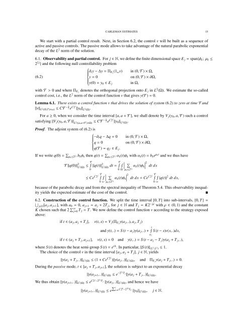
We start with a partial control result. Next, in Section 6.2, the control v will be built as a sequence of
active and passive controls. The passive mode allows to take advantage of the natural parabolic exponential
decay of the L 2 norm of the solution.
6.1. Observability and partial control. For j ∈ N, we define the finite dimensional space E j = span{φ k ; µ k ≤
2 2 j } and the following null controllability problem
⎧
∂ t y − ∆y = Π E j
(1 ω v) in (0, T ) × Ω,
⎪⎨
(6.2)
y = 0
on (0, T ) × ∂Ω,
⎪⎩ y(0) = y 0 ∈ E j in Ω,
with T > 0 and where Π E j
denotes the orthogonal projection onto E j in L 2 (Ω). We estimate the so-called
control cost, i.e., the L 2 norm of the control function v that gives y(T ) = 0.
Lemma 6.1. There exists a control function v that drives the solution of system (6.2) to zero at time T and
‖v‖ L 2 ((0,T)×ω) ≤ CT − 1 2 e C2 j ‖y 0 ‖ L 2 (Ω).
For a ≥ 0, when we consider the time interval [a, a + T ], we shall denote by V j (y 0 , a, T ) such a control
satisfying ‖V j (y 0 , a, T )‖ L 2 ((a,a+T )×Ω) ≤ CT − 1 2 e C2 j ‖y 0 ‖ L 2 (Ω).
Proof. The adjoint system of (6.2) is
⎧
−∂ t q − ∆q = 0 in (0, T ) × Ω,
⎪⎨
q = 0
on (0, T ) × ∂Ω,
⎪⎩ q(T ) = q f ∈ E j .
If we write q(0) = ∑ µ k ≤2 b kφ 2 j k then q(t) = ∑ µ k ≤2 α k(t)φ 2 j k with α k (t) = b k e µ kt and we thus have
T ‖q(0)‖ 2 L 2 (Ω) ≤ T ∫ ‖q(t)‖ 2 L 2 (Ω) dt = T ∫ ∫
∑
∣ ∣∣∣ 2
∣ α k (t)φ k dt dx
0
0 Ω µ k ≤2 2 j
≤ Ce C2 j T
∫ ∫
∑
∣ ∣∣∣ 2
∣ α k (t)φ k dt dx = Ce
C2 j T
∫ ∫ |q(t)| 2 dt dx,
0 ω µ k ≤2 2 j 0 ω
because of the parabolic decay and from the spectral inequality of Theorem 5.4. This observability inequality
yields the expected estimate of the cost of the control.
6.2. Construction of the control function. We split the time interval [0, T] into sub-intervals, [0, T] =
⋃
j∈N[a j , a j+1 ], with a 0 = 0, a j+1 = a j + 2T j , for j ∈ N and T j = K2 − jρ with ρ ∈ (0, 1) and the constant
K chosen such that 2 ∑ ∞
j=0 T j = T. We now define the control function v according to the strategy exposed
above:
if t ∈ (a j , a j + T j ], v(t, x) = V j (Π E j
y(a j , .), a j , T j )
and y(t, .) = S (t − a j )y(a j , .) + t
∫
a j
S (t − s)v(s, .)ds,
if t ∈ (a j + T j , a j+1 ], v(t, x) = 0 and y(t, .) = S (t − a j − T j )y(a j + T j , .),
where S (t) denotes the heat semi-group S (t) = e t∆ . In particular, ‖S (t)‖ (L 2 ,L 2 ) ≤ 1.
The choice of the control v in the time interval [a j , a j + T j ], j ∈ N, yields
‖y(a j + T j , .)‖ L 2 (Ω) ≤ (1 + Ce C2 j )‖y(a j , .)‖ L 2 (Ω), and Π E j
y(a j + T j , .) = 0.
During the passive mode, t ∈ [a j + T j , a j+1 ], the solution is subject to an exponential decay
‖y(a j+1 , .)‖ L 2 (Ω) ≤ e −22 j T j
‖y(a j + T j , .)‖ L 2 (Ω).
We thus obtain ‖y(a j+1 , .)‖ L 2 (Ω) ≤ e C2 j −2 2 j T j
‖y(a j , .)‖ L 2 (Ω), and hence we have
‖y(a j+1 , .)‖ L 2 (Ω) ≤ e∑ j
k=0 C2k −2 2k T k
‖y 0 ‖ L 2 (Ω), j ∈ N.