Dynamic Hedging with Stochastic Differential Utility

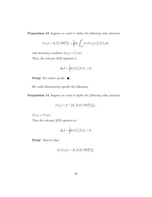
Proposition 13 Suppose we want to define the following value function
Z
£ ¡ ¢¤
J (z t )=E t U W
θt 1 T
T +
2 E t k (J (z s )) Jz 0 s
ΣJ zs ds,
s≥t
with boundary condition J(z T )=U (w).
Then, the relevant HJB equation is
A d J + 1 2 k(J)J 0 z t
ΣJ zt =0.
Proof. See earlier proofs.
We could alternatively specify the following:
Proposition 14 Suppose we want to define the following value function
J (z t )=h ¡ £ ¡ ¡ ¢¢¤¢ −1 E t h U W
θt
T ,
J(z T )=U (w).
Then the relevant HJB equation is:
A d J + 1 2 k(J)J 0 z t
ΣJ zt =0.
Proof. Observe that:
£ ¡ ¡ ¢¢¤
h (J (z t )) = E t h U W
θt
T
42