zmap a tool for analyses of seismicity patterns typical applications ...

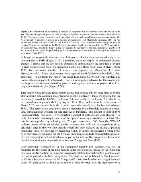
Figure 2.5: Comparison of the rates as a function of magnitude for two periods, which are printed at the
top. The rate change took place in 1995.5 along the Parkfield segment of the San Andreas fault (35.3° to
36.4°). The numbers are normalized by the duration of the periods. (A) Frequency-magnitude curve. (B)
Non-cumulative numbers of events as a function of magnitude. (C) Magnitude signature. (D) The rate
comparison before and after 1995.5 in the usual FMD format. The three lines below the graph give the
results of fits by two methods to the FMD of the first period (black) and the result by the WLS method for
the second period. Inside the figure, at the top, appears the summary of the data, numbers of events used,
and b-values found. Also, the probability, p, that the two sets are drawn from an indistinguishable common
set is given (Utsu, 1992).
Although the magnitude signature is an informative plot for the experienced analyst, the
non-cumulative FMD (Figure 2.5B) is probably the most helpful to understand the rate
change. It shows that the two periods experienced approximately the same rate of events
in their respective top-reporting magnitude bands, only, these bands were shifted. Before
1995, the maximum number of events was reported at Mmax(pre)=1.0, after
Mmax(post)=1.2. Many more events were reported for 0.7≤M≤0.9 before 1995.5 than
afterward. In contrast, the rate in the magnitude band 1.2≤M≤1.6 was substantially
lower, before compared to afterward. This type of opposite behavior for the smaller and
the larger events is demonstrated by positive and negative peaks on opposite sides of the
magnitude signature plot (Figure 2.5C).
That nature would produce fewer larger events, but balance this by more smaller events
after a certain date without a major tectonic event is not likely. Thus, we propose that the
rate change found by GENAS in Figure 2.4, and analyzed in Figure 2.5, should be
interpreted as a magnitude shift (e.g. Wyss, 1991). If we look at it in the presentation of
Figure 2.5D, we see that it is also a mild magnitude stretch (e.g. Zuniga and Wiemer,
1999). This result is not good news, since it happened in the Parkfield catalog at a recent
date, introducing an obstacle for rate analyses at Parkfield. The amount of shift in 1995
is approximately +0.2 units. Even though the amount of shift appears to be close to +0.2
units, it would be necessary to determine the optimal value by a quantitative method. This
can be accomplished by selecting the "Compare two rates (fit)" from the "ZTools"
pulldown menu of the cumulative number window. You will start a comparison of the
seismicity rates in the two time periods which this time includes the fitting of possible
magnitude shifts, or stretches of magnitude scale, by means of synthetic b-value plots.
Also provided are estimates for the b-value, minimum magnitude of completeness, mean
rate for each period, and z-test values comparing the rates of the two periods. For a more
detailed description on magnitude stretches, see Zuniga and Wyss (1995).
After selecting "Compare-fit" in the cumulative number plot window, you will be
prompted for the limits of the time periods under investigation, just as for the “Compare
two rates (no-fit)” option. A frequency-magnitude relation (normalized to a year) for each
interval is plotted with different symbols. The first interval is labeled as "background",
while the subsequent interval is the "foreground". You should select two magnitude endpoints
for each curve to obtain an estimated b-value for each interval; these have to be
17