zmap a tool for analyses of seismicity patterns typical applications ...

CHAPTER III
Measuring Changes of Seismicity Rate
Precondition: You have already selected the part of an earthquake catalog that is
reasonably homogeneous in space, time and magnitude band. All inadequate parts of the
catalog and explosions have been removed.
Measuring a Local Rate Change: Suppose you have selected earthquakes from some
volume, and, displaying it in a cumulative number curve, you notice a change in slope
(Figure 3.1a), which you want to measure.
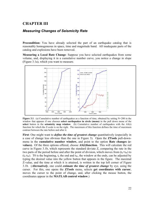
Figure 3.1: (a) Cumulative number of earthquakes as a function of time, obtained by setting N=200 in the
window that appears if one chooses select earthquakes in circle (menu) in the pull down menu of the
select button in the seismicity map window. (b) Cumulative number of earthquakes with the AS(t)
function for which the Z-scale is on the right. The maximum of this function defines the time of maximum
contrast between the rate before and after it.
First: One might want to define the time of greatest change quantitatively (especially in
a case of change less obvious than the one in Figure 3). Open the ZTools pull-downmenu
in the cumulative number window, and point to the option Rate changes (zvalues).
Of the three options offered, choose AS(t)function. This will calculate the red
curve in Figure 3.1b, which represents the standard deviate Z, comparing the rate in the
two parts of the period before and after the point of division, which moves from (t0+tW) to
(te-tW). T0 is the beginning, te the end and tW, the window at the ends, can be adjusted by
typing the desired value into the yellow button that appears in the figure. The maximal
Z-value, and the time at which it is attained, is written in the top left corner of Figure
3.1b. (Alternatively, one could estimate the time of greatest change by eye, using the
curser. For this, one opens the ZTools menu, selects get coordinates with cursor,
moves the cursor to the point of change, and, after clicking the mouse button, the
coordinates appear in the MATLAB control window.)
22