heat transfer limit due to pressure drop of a loop ... - LEPTEN

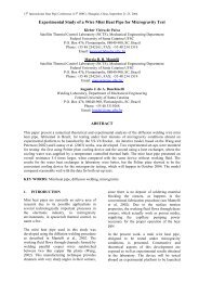
15th International Heat Pipe Conference (15th IHPC)
Clemson, USA, April 25-30, 2010
HEAT TRANSFER LIMIT DUE TO PRESSURE DROP OF A LOOP THERMOSYPHON
Milanez F. H., Mantelli M. B.H.
Mechanical Engineering Dept., Federal University of Santa Catarina
Florianopolis, SC, Brazil, 88040-900
Phone: +55 48 3721 9937, Fax: +55 48 3721 7615
milanez@labtucal.ufsc.br, marcia@emc.ufsc.br
ABSTRACT
This work presents theoretical and experimental studies on the heat transfer limit due to pressure drop of loop
thermosyphons. This limit is reached when the condensate return level reaches the end of the condenser. Any
further increase in the heat transfer rate makes the condensate to block part of the condenser, increasing the
overall thermal resistance. No references were found on this subject in the literature. A model based on literature
models and correlations for pressure drop in single and two-phase flow is developed here to predict the heat
transfer limit due to pressure drop. A loop thermosyphon prototype was built and tested. The obtained data is
relatively well predicted by the proposed model, showing that it can be used as a design tool for loop
thermosyphons.
KEY WORDS: Loop Thermosyphon, Pressure Drop, Two-phase Flow
1. INTRODUCTION
Loop thermosyphon heat exchangers, also known as
separated heat pipes, have been successfully applied
in industrial waste heat recovery systems. Figure 2
presents a schematic drawing of a typical loop
thermosyphon heat exchanger. Both the evaporator
and the condenser are geometrically very similar.
They consist of two horizontal headers (upper and
lower) connected by several vertical tubes in parallel.
The vapor line coming from the evaporator is
connected to the upper header. As vapor condenses,
the liquid flows by gravity to the lower header, which
is connected back to the evaporator.
Petrobras, the Brazilian Petroleum Company,
employs several large asphalt storage tanks in their
plants with a capacity of more than a thousand tons.
In order to keep the asphalt at the required
temperature level of 140°C, the tanks are equipped
with steam coils placed at the bottom. The steam is
available from a 10 bar boiler that is responsible for
all the steam used inside the Plant. As the boiler is
located far from the tanks, large heat losses are
present.
A loop thermosyphon is being developed for
application in asphalt tanks heating. The objective of
the thermosyphon is to replace the actual heating
system. The condenser of the loop thermosyphon is
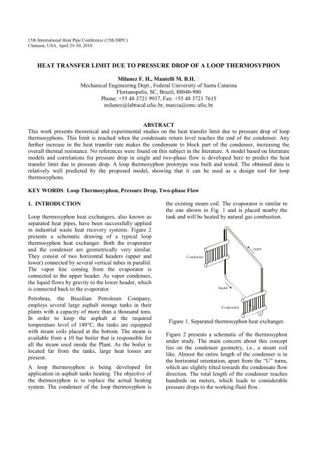
the existing steam coil. The evaporator is similar to
the one shown in Fig. 1 and is placed nearby the
tank and will be heated by natural gas combustion.
Condenser
liquid
Evaporator
vapor
Figure 1. Separated thermosyphon heat exchanger.
Figure 2 presents a schematic of the thermosyphon
under study. The main concern about this concept
lies on the condenser geometry, i.e., a steam coil
like. Almost the entire length of the condenser is in
the horizontal orientation, apart from the “U” turns,
which are slightly tilted towards the condensate flow
direction. The total length of the condenser reaches
hundreds on meters, which leads to considerable
pressure drops to the working fluid flow.

The flow of working fluid inside a loop
thermosyphon is associated to a pressure drop. The
larger is the heat transfer rate through the loop
thermosyphon, the larger is the working fluid velocity
and the larger is the pressure drop. The pressure drop
due to the working fluid flow must be compensated
by a hydraulic head between evaporator and
condenser. Figure 2 presents a schematic of this
phenomenon. The hydraulic head h is the difference
between the liquid levels in the evaporator and in the
condensate return line. The maximum allowable
difference is h max , i.e., the vertical distance between
evaporator liquid pool surface and condenser bottom.
When the thermosyphon is at the heat transfer limit
due to pressure drop, h=h max . Any further increase in
the heat transfer rate makes the condensate to block
part of the condenser. A further increase in the heat
transfer rate leads to h>h max (see Fig. 3). The
thermosyphon thermal resistance increases because
the available are for two-phase heat transfer
increases. That is because only the portion of the
condenser that can be reached by the vapor is
effective for heat transfer. The portion of the
condenser that is filled with condensate no longer
operates in two-phase heat transfer mode.
Figure 2. Hydraulic head h in a loop thermosyphon
This work presents both theoretical and experimental
studies on the heat transfer limit of loopthermosyphons.
The main objective is to develop a
model to help the design of loop thermosyphons.
Under normal operation, the thermosyphon should
operate in the condition shown in Fig.3, i.e., bellow
the heat transfer limit due to pressure drop.
Figure 3. Loop thermosyphon beyond the pressure
drop limit
2. THEORETICAL ANALYSIS
When the hydraulic head due to working fluid flow
pressure drop is equal to the vertical distance
between the liquid pool level at the evaporator and
the bottom of the condenser, the loop thermosyphon
is reaching a heat transfer limit. In this work, this
limit is called here “the heat transfer limit due to
pressure drop”. Any increase in the heat transfer rate
makes the condensate level to fill up the condenser,
blocking heat transfer and leading to the system’s
failure. A theoretical model to predict the heat
transfer limit due to pressure drop is developed here.
The model is based on literature correlations and
models for viscous fluid flow pressure drop.
The total pressure drop ∆P t of the working fluid flow
is related to the hydraulic head h through the
following expression:
( ρ − ρ ) g h
∆ P =
(1)
t
l
where g=9,81 m/s 2 . In this equation, the pressure
gradient resulting from momentum variation at the
liquid-vapor interfaces were neglected.
The total pressure drop ∆P t is the summation of the
v

pressure drops due to fluid flow at the evaporator
∆P evap , vapor line ∆P v , condenser ∆P cond and
condensate return line ∆P l , i.e.:
∆ P = ∆P
+ ∆P
+ ∆P
+ ∆P
(2)
t
evap
v
cond
If the vapor line is well insulated so there is no
condensation, the flow is single-phase (vapor). When
the thermosyphon is operating at the limit, the
condensate return line is filled with liquid (h=h max ),
and the flow in the condensate return line is also
single-phase. The single-phase flow pressure drop
can be calculated form classical fluid flow textbooks
(Fox & McDonnald, 1988), such as:
2
Le
ρ V
∆ P = f
(3)
d 2
i
For smooth pipes, the friction coefficient can be
computed as:
0.316
f =
(4)
0.25
Re
where Re, the Reynolds number is defined as:
ρVD 4 q
Re ≡ =
(5)
µ h lv
π d i
µ
The equivalent length L e , appearing in Eq. (3) is the
summation of the vapor line total length and the
equivalent length of the bends, valves and other
components of the circuit. The other two components
of the pressure drop in Eq. (3), in the evaporator and
in the condenser, are more complex due to the twophase
nature of the flow.
The pressure drop in two-phase fluid flow has been
the subject of several researches [2,3,4]. Two
classical models have been developed: homogeneous
model and separated model. In the homogenous
model, the two phases flow at the same velocity. In
the separated model, there is a non-zero relative
velocity (shear) between the phases. The results of
two models are presented in the following sections.
More details are provided in the references.
2.1 Homogeneous model
In the development of the homogeneous model for
two-phase flow pressure drop it is assumed that the
flow is one-dimensional and the liquid and vapor
velocities are the same. In other words, the two
phases are replaced by a hypothetical fluid with
homogenous properties throughout all the points of
l
the flow. According to Collier & Thome (1994), the
pressure gradient is calculated as:
−
⎪⎧
2 fTPG
⎨
dP
=
⎪⎩
ρldi
dz
where:
2
⎡ ⎛ v ⎤
lv
⎞ g sin Ω
⎢1
+ x
⎜
⎟⎥
+
⎣ ⎝ vl
⎠⎦
l lv
⎛ dv ⎞
⎜ +
2 v
1 G x ⎟
⎝ dP ⎠
( v + x v )
+ G
2
dx ⎪⎫
vlv
⎬
dz ⎪ ⎭
(6)
m
G = &
(7)
A
q
m & =
(8)
h lv
m&
v
x = (9)
m&
−0,25
⎛ G di
⎞
f
TP
= 0,079⎜
⎟
(10)
⎝ µ ⎠
The literature presents several definition for the
equivalent viscosity µ . In this work, two models
found in Wallis (1969) are used:
v
( x) l
( 1−
x)
µ = x µ + 1 − µ (Cicchitti) (11)
1 x
= +
µ µ
v
µ
l
(McAdams) (12)
The second term in the denominator of Eq. (6) is
related to the vapor compressibility and is normally
neglected, so the denominator is approximately one.
For the geometry of Fig. 3, the quality x [ ] is one at
the condenser inlet and zero at the exit. Between the
two points, the variation is assumed to be linear
because the heat flux, and consequently the
condensation rate, is uniform along the condenser
length, i.e.:
z
x = 1 −
(13)
L cond
The condenser pressure drop is finally computed as:
∆P
cond
=
∫
0
L cond
dP
dz
dz
(14)
where L cond [m] is the total condenser length,
including the equivalent lengths of the “U” bends. In
this work, the equivalent length of one “U” turn is
assumed to be 50 times the internal diameter of the

tube. This value was encountered in Fox &
McDonnald (1988) for single-phase flow. Despite
this is two-phase flow, the above value was used
because of the lack of specific values.
The set of equations above are solved numerically to
obtain the total pressure drop of the condenser. The
condenser total length, including the equivalent
length of the “U” bends, is divided in 100 parts. The
pressure drop of each part is calculated considering
constant values of the quantities given by Eqs. (6)
and (10) to (13) within each part.
2.2 Separated model
As already mentioned, in the separated model, the
two phases flow at different speeds. According to
Collier and Thome (1994), the expression for the
local pressure gradient is:
( 1−
x)
⎛
2 2
⎡
⎤
⎜ 2 2 f
lG
φl
⎢
⎥ +
dP 1
⎜ ⎣ ρldi
⎦
− = ⎜
dz Λ ⎜ ⎪⎧
2 dx ⎡ 2x
2 1
⎜G
⎨⎢
−
dz
⎝ ⎪⎩ ⎣ ρv
α ρv
[( 1−α
) ρ + αρ ]
( − x)
( 1−α
)
l
v
⎤ dα
⎡
⎥ + ⎢
⎦ dx ⎣ ρ
g sin Ω +
2
2
( 1−
x)
x ⎤⎪⎫
− ⎥⎬
( − ) ⎦
⎟ ⎪⎭
⎟⎟⎟⎟⎟ 2 2
1 α ρvα
v
⎠
(15)
where Λ≈1, which means the vapor compressibility
and can be neglected (Carey, 1992), similarly to the
homogeneous model. The liquid friction coefficient is
calculated in a similar fashion to Eq. (10), that is:
f
l
⎡G
= 0,079⎢
⎣
( 1−
x)
µ
l
d
⎤
⎥
⎦
i
−0,25
⎞
(16)
Several methods are presented in the literature to
determine the two-phase multiplier and the void
fraction, most of them of empirical nature. Carey
(1992) presents the correlations developed by
Lockhart and Martinelli for these quantities:
where:
1/ 2
⎛ C 1 ⎞
φ
l
= ⎜1+
+
2
⎟ (17)
⎝ X X ⎠
0,71 −
( 1+
0,28 ) 1
α = X
(18)
X
2
⎛ dP ⎞
⎜ ⎟
⎝ dz ⎠
=
⎛ dP ⎞
⎜ ⎟
⎝ dz ⎠
l
v
(19)
This quantity is called the Martinelli Parameter,
which is the ratio between the pressure drop that
would occur if only the liquid phase was present and
the pressure drop that would occur if only the vapor
phase was present. These two pressure drops are
evaluated using equations for single phase flow:
⎛ dP ⎞
⎜ ⎟
⎝ dz ⎠
l
⎛ dP ⎞
⎜ ⎟
⎝ dz ⎠
v
( x)
2 flG
2 1−
= −
ρ d
2
= −
v
l
i
i
2
fvG
x
ρ d
2
2
(20)
(21)
The constant C which appears in Eq. (17) depends
on the nature of the flows:
• C=20 for turbulent liquid and vapor flow
• C=12 for turbulent vapor and laminar liquid
flow
• C=10 for laminar vapor and turbulent liquid
flow
• C=5 for laminar liquid and vapor flow
Carey (1992) present other models for the two-phase
multiplier. Wallis (1969) proposes a model where
liquid and vapor flow in separated tubes with distinct
diameters, but with the same total area as the actual
tube. Furthermore, the pressure drops of the two
flows must be equal to the pressure drop of the
actual flow. For turbulent flow, it yields:
19
16
16
⎡ ⎤
1 19
⎢ ⎛ ⎞
φ 1 ⎥
l
= + ⎜ ⎟
(22)
⎢ ⎝ X ⎠ ⎥
⎣ ⎦
Finally, the friction coefficient for the liquid phase is
calculated with Eq. (16) while the friction coefficient
for the vapor phase is calculated with:
f
v
⎡Gxd
= 0,079 ⎢
⎣ µ
v
⎤
⎥
⎦
i
−0,25
(23)
Similarly to the homogenous model, the total length
of the condenser is divided in 100 parts and the total
pressure drop is calculated numerically as the
summation of the pressure drops of the 100 parts.
Within each part the quantities given by Eqs. (13)
and (15) to (23).

3. EXPERIMENTAL STUDY
3.1. Experimental Set-Up
A stainless steel-water loop thermosyphon prototype
was built and tested for the heat transfer limit due to
pressure drop. The condenser is a stainless-steel 6
mm internal diameter and 11 m horizontal tube with
several “U” bends. Figure 4 shows a schematic of the
experimental set-up. The prototype maximum
allowable hydraulic head (Fig. 2) is h max =2 m. The
evaporator is a horizontal cylinder with cartridge
heaters immersed in the liquid pool. The heat transfer
is computed as the electric power input to the heaters
minus the thermal insulation losses.
The condenser is inserted in a controlled thermal bath
with (ethylene-glycol) in the forced convection. The
temperature of the thermal fluid is controlled through
a LAUDA® PR855 controlled temperature thermal
bath.
The evaporator of the model is made of a SS 316
horizontal tube with 100 mm i.d. and 400 mm long.
The working fluid is distillated water and the filling
ratio is 80% of the evaporator volume. The vapor line
is connected to the top of the horizontal cylinder,
while the liquid return line is connected to the side of
the cylinder, below the liquid pool level. Heat is
provided by eight 20 mm o.d. cartridge type electrical
heaters immersed in the liquid pool. The entire
system is insulated with glass wool, with the thermal
losses estimated in 100 W. By measuring the
electrical resistance and the current, the heat power
input could be accurately assessed.
The condenser could also be tilted with respect to
the horizontal position (see tilt angle θ in Fig. 4).
However, preliminary measurements showed the
system is not greatly affected by this angle. This is
because most part of the condenser remains in
horizontal orientation, regardless of the tilt angle.
Only the “U” bends experience change in the
orientation as the tilt angle is varied. All the tests
presented here are for θ= 13°.
The condenser was instrumented with seven K-type
thermocouples distributed evenly over its length.
The first thermocouple was placed 50 mm from the
start of the condenser. The seventh thermocouple
was placed 50 mm from the end of the condenser.
Figure 5 present the thermocouple distribution. The
vapor line was instrumented with one K-type
thermocouple next to the evaporator exit. The
evaporator was instrumented with two K-type
thermocouples: one immersed in the liquid pool and
one immersed in the vapor space above the liquid
pool. The controlled thermal bath was measured by
two K-type thermocouples, one at the inlet and one
at the outlet. The temperature, voltage and current
were measured with a HP 3947-A® Data
Acquisition System connected to a personal
computed, which stored the data for further
treatment.
vapor
condenser
θ
liquid
evaporator
controled
temperature
bath
Figure 4. Experimental set-up.
Figure 5. Thermocouple distribution.

3.2. Tests Procedure
The heater was turned on starting from the thermal
equilibrium with the ambient. The power input was
first set to 1000 W. After the system reached steady
state, the power input was increased by steps of 500
W. In each power step, the system was left to reach
steady state. Before the system reached the heat
transfer limit due to pressure drop, the condenser
thermocouples give virtually the same reading, which
is above the controlled thermal bath, showing the
vapor reached the condenser entire length and it is
transferring heat to the thermal bath. After the system
exceeded the limit, the condensate level floods part of
the condenser (Fig. 4). This can be easily noticed by
inspecting the thermocouple readings, which give the
same readings as the thermocouples of the thermal
bath. In this case, that part of the condenser is
inactive for heat transfer. At this point, the test was
finished and the heater was turned off.
This procedure was repeated for several mean
temperature levels of the thermosyphon. The mean
temperature level was varied by changing the
temperature level of the controlled thermal bath.
3.3. Experimental Uncertainty
After calibration of the system, the uncertainty in
temperature measurement is ±0.60°C in the range of
temperatures of interest. The uncertainty in voltage
measurement is ±0.1%, and the uncertainty of the
heater electrical resistance value was found to be
±4%.
The separated model with the two-phase multiplier
computed using Wallis’ model yielded the best
agreement with the measured data. The other
models/correlations predicted lower values for the
heat transfer limit due to pressure drop.
In order to understand how the authors knew
whether the thermosyphon reached the heat transfer
limit or not, let’s examine Fig. 7. It presents the
temperature readings as a function of time for the
controlled thermal bath set at 150°C. As one can see,
the evaporator temperatures (103 and 104, Fig. 5)
are very close together and approximately 20°C
above the condenser temperatures (106 to 112). The
condenser temperature readings also relatively close
to each other, with the maximum temperature
difference of approximately 4°C. The difference of
temperature readings between the first (106) and the
last (112) condenser temperature is less than 0.8°C,
which shows that the condenser cooling is
approximately isothermal. For time

temperature [°C]
condenser (112), which means the system exceeded
the heat transfer limit de to pressure drop. Therefore
one concludes that the limit lies between heat transfer
rates of 3.9 kW and 4.4 kW. The measured heat
transfer limit is defined here as the average of the two
values, i.e., approximately 3.15kW. The limit was
reached when the thermosyphon mean temperature
was 178°C (average of the thermocouple readings
from 103 to 112).
All the data points presented in the graph of Fig. 6
were obtained using the procedure described above.
The uncertainty of this procedure is 500W, which is
the test power step. The amplitude of the error bar is
therefore 500W. The error bar then indicates that the
limit could be actually anywhere within that range.
180
175
170
165
160
155
100 102 104 106 108 110 112 114 116
time [min]
thermocouple 112
Figure 7. Temperature reading as a function of time.
5. CONCLUSIONS
This work presented theoretical and experimental
studies on the heat transfer limit due to pressure drop
of loop thermosyphons. This limit is specially
important for large pressure drops systems, such as
heating systems where the condenser is a long steam
coil. When the thermosyphon exceeds this limit, the
condensate blocks part of the condenser, increasing
the overall thermal resistance.
A model is proposed here, which is based on
literature models and correlations for pressure drop in
both single and two-phase flows. A prototype was
built and tested for the heat transfer limit due to
pressure drop. The data is relatively well predicted by
the proposed model. The model can then be
employed as a loop thermosyphon design tool, so the
thermosyphon can operate safely bellow this limit.
103
104
105
106
107
108
109
110
111
112
113
114
115
116
NOMENCLATURE
A cross sectional area [m 2 ]
C constant (see Eq. 18)
d i inner diameter [m]
f friction coefficient [ ]
G mass flux [kg/s.m 2 ]
h hydraulic head
h lv latent heat of vaporization [J/kg]
L length [m]
m& mass flow rate [kg/s]
P thermodynamic pressure[Pa]
q heat transfer rate [W]
Re Reynolds number
v specific volume (=1/ρ) [m³/kg]
V velocity [m/s]
x vapor quality [ ]
X 2 Martinelli Parameter
z coordinate axis along the flow[m]
Subscripts
evap evaporator
cond condenser
e equivalent
l liquid
v vapor
TP two-phase
Greek letters
α void fraction ( = A )[ ]
A v
φ
l
two-phase multiplier [ ]
µ absolute viscosity [Pa.s]
ρ density [kg/m³]
Ω tube tilt angle [°]
ACKNOWLEDGEMENT
The authors would like to acknowledge the support
of PETROBRAS, the Brazilian Petroleum Company,
during this research.
REFERENCES
1. Fox, R. W. & McDonald, A. T., Introdução à
Mecânica dos Fluidos, Guanabara Koogan, 3 a .
Edição, Rio de Janeiro, 1988.
2. Collier, J. G. and Thome, J. R., Convective
Boiling and Condensation, Clarendon Press, 3 rd
Edition, Oxford, 1994.
3. Wallis, G. B., One-dimensional Two-phase
Flow, McGraw-Hill, 1969.
4. Carey, V. P., Liquid-Vapor Phase-Change
Phenomena, Taylor & Francis, 1992.