A kinetic approach in nonlinear parabolic problems ... - ENS Cachan
A kinetic approach in nonlinear parabolic problems ... - ENS Cachan
A kinetic approach in nonlinear parabolic problems ... - ENS Cachan

You also want an ePaper? Increase the reach of your titles
YUMPU automatically turns print PDFs into web optimized ePapers that Google loves.
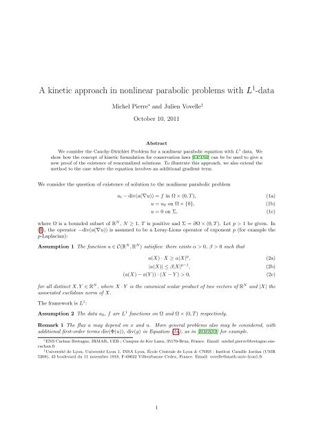
A <strong>k<strong>in</strong>etic</strong> <strong>approach</strong> <strong>in</strong> nonl<strong>in</strong>ear <strong>parabolic</strong> <strong>problems</strong> with L 1 -data<br />
Michel Pierre ∗ and Julien Vovelle †<br />
October 10, 2011<br />
Abstract<br />
We consider the Cauchy-Dirichlet Problem for a nonl<strong>in</strong>ear <strong>parabolic</strong> equation with L 1 data. We<br />
show how the concept of <strong>k<strong>in</strong>etic</strong> formulation for conservation laws [LPT94] can be be used to give a<br />
new proof of the existence of renormalized solutions. To illustrate this <strong>approach</strong>, we also extend the<br />
method to the case where the equation <strong>in</strong>volves an additional gradient term.<br />
We consider the question of existence of solution to the nonl<strong>in</strong>ear <strong>parabolic</strong> problem<br />
u t − div(a(∇u)) = f <strong>in</strong> Ω × (0, T ),<br />
u = u 0 on Ω × {0},<br />
u = 0 on Σ,<br />
(1a)<br />
(1b)<br />
(1c)<br />
where Ω is a bounded subset of R N , N ≥ 1, T is positive and Σ = ∂Ω × (0, T ). Let p > 1 be given. In<br />
(1), the operator −div(a(∇u)) is assumed to be a Leray-Lions operator of exponent p (for example the<br />
p-Laplacian):<br />
Assumption 1 The function a ∈ C(R N , R N ) satisfies: there exists α > 0, β > 0 such that<br />
a(X) · X ≥ α|X| p ,<br />
|a(X)| ≤ β|X| p−1 ,<br />
(a(X) − a(Y )) · (X − Y ) > 0,<br />
(2a)<br />
(2b)<br />
(2c)<br />
for all dist<strong>in</strong>ct X, Y ∈ R N , where X · Y is the canonical scalar product of two vectors of R N and |X| the<br />
associated euclidean norm of X.<br />
The framework is L 1 :<br />
Assumption 2 The data u 0 , f are L 1 functions on Ω and Ω × (0, T ) respectively.<br />
Remark 1 The flux a may depend on x and u. More general <strong>problems</strong> also may be considered, with<br />
additional first-order terms div(Φ(u)), div(g) <strong>in</strong> Equation (1a), as <strong>in</strong> [BMR01] for example.<br />
∗ <strong>ENS</strong> <strong>Cachan</strong> Bretagne, IRMAR, UEB ; Campus de Ker Lann, 35170-Bruz, France. Email: michel.pierre@bretagne.enscachan.fr<br />
† Université de Lyon, Université Lyon 1, INSA Lyon, École Centrale de Lyon & CNRS ; Institut Camille Jordan (UMR<br />
5208), 43 boulevard du 11 novembre 1918, F-69622 Villeurbanne Cedex, France. Email: vovelle@math.univ-lyon1.fr<br />
1
1 Introduction<br />
The existence of solution (precisely, of renormalized solution, see Def<strong>in</strong>ition 1 below) to Problem (1) or<br />
quite more general <strong>problems</strong> has already been proved: we refer <strong>in</strong> particular to the paper by Blanchard,<br />
Murat, Redwane [BMR01]. Our purpose here is to give a new proof of this fact. The cornerstone <strong>in</strong><br />
the proof of existence of solution (by means of a process of approximation) of such a nonl<strong>in</strong>ear <strong>parabolic</strong><br />
Problem as (1) is the proof of the strong convergence of the gradient. We give a new method (<strong>in</strong>spired from<br />
the <strong>k<strong>in</strong>etic</strong> formulation of conservation laws developed by Perthame and coauthors [LPT94, Per02, CP03])<br />
to prove this result.<br />
Let us briefly summarize how and <strong>in</strong> which context the question of strong convergence of the gradient<br />
occurs: first, as soon as the problem under consideration <strong>in</strong>volves a nonl<strong>in</strong>ear function of the gradient.<br />
This is for example the case of the follow<strong>in</strong>g <strong>problems</strong>:<br />
or<br />
− ∆u + γ(u)|∇u| 2 = g <strong>in</strong> Ω, u = 0 on ∂Ω, (3)<br />
− div(a(∇u)) = g <strong>in</strong> Ω, u = 0 on ∂Ω, (4)<br />
with given right-hand side g ∈ L 2 (Ω), where a satisfies (2) with p = 2, and γ is a bounded cont<strong>in</strong>uous<br />
function satisfy<strong>in</strong>g the sign condition uγ(u) ≥ 0 for all u ∈ R. Indeed, <strong>in</strong> order to prove existence of<br />
a solution (<strong>in</strong> H0 1 (Ω)) to (3) or (4), it is usual to prove existence by approximation, for example by<br />
Galerk<strong>in</strong> approximation, thus for a set of data g n converg<strong>in</strong>g to g. Then weak convergence <strong>in</strong> H0<br />
1 of<br />
possibly a subsequence of u n , the solution with datum g n , although easily obta<strong>in</strong>ed by uniform estimate<br />
on ‖u n ‖ H1 (Ω), is not enough to pass to the limit: one has to prove 1 the strong convergence of the gradient<br />
∇u n . This is done by use of monotonicity methods. We refer to [M<strong>in</strong>63, Bro63, LL65], and [Eva98] for<br />
a brief explanation of the technique.<br />
Nonl<strong>in</strong>ear expressions of the gradient also occur after renormalization of an elliptic or <strong>parabolic</strong> equation.<br />
Note actually that they occur even if the orig<strong>in</strong>al equation is l<strong>in</strong>ear. Nevertheless, renormalization<br />
for elliptic or <strong>parabolic</strong> equation has been <strong>in</strong>troduced to deal with nonl<strong>in</strong>ear equations with data of<br />
low regularity, and as a consequence, once renormalized, the equation <strong>in</strong>volves at least two nonl<strong>in</strong>ear<br />
expressions of the gradient (see, e.g. Eq. (6) below). In any case, it will be necessary to prove the strong<br />
convergence of the (truncates of) the gradient <strong>in</strong> order to get existence of a solution by approximation.<br />
We give a new proof of the strong convergence of the gradient by use of an equation on the characteristic<br />
function on the level sets of the unknown, similar to the <strong>k<strong>in</strong>etic</strong> formulation for conservation<br />
laws <strong>in</strong>troduced <strong>in</strong> [LPT94] (see also [Per02] and [CP03] concern<strong>in</strong>g the <strong>k<strong>in</strong>etic</strong> formulation of secondorder<br />
conservation laws). We <strong>in</strong>tend to use it to study certa<strong>in</strong> systems of reaction-diffusion equations (a<br />
forthcom<strong>in</strong>g paper).<br />
Let us conclude this <strong>in</strong>troduction by a few words about the concept of renormalized solutions. Introduced<br />
by DiPerna and Lions for the study of ord<strong>in</strong>ary differential equations and Boltzmann Equation [DL89b,<br />
DL89a], it has been extended to nonl<strong>in</strong>ear elliptic equations <strong>in</strong> [BGDM93] <strong>in</strong> parallel with the equivalent<br />
notion of entropy solution [BBG + 95] and has been extended to nonl<strong>in</strong>ear <strong>parabolic</strong> equations <strong>in</strong> [Bla93,<br />
BMR01, Lio96], <strong>in</strong> parallel with the equivalent notion of entropy solution [Pri97]. It has also been<br />
extended to first-order conservation laws [BCW00, PV03].<br />
The problem of strong convergence of the gradient, hence the question of existence of solution, has <strong>in</strong>itially<br />
be solved by the method of M<strong>in</strong>ty-Browder and Leray-Lions [M<strong>in</strong>63, Bro63, LL65], then extended to the<br />
case of nonl<strong>in</strong>ear elliptic, then <strong>parabolic</strong> equations with less and less regular data by several methods,<br />
see, e.g. [BG92a, BM92, BGM93, BGDM93, DMMOP97, BDGO99, DMMOP99, BMR01, BP05]. Note<br />
that this list of references to some works <strong>in</strong> the field of renormalized solutions for elliptic and <strong>parabolic</strong><br />
equations is far from be<strong>in</strong>g complete.<br />
1 Actually, <strong>in</strong> Problem (4) it is sufficient to obta<strong>in</strong> the weak convergence of (a(∇u n)) to a(∇u), see Remark 3<br />
2
The paper is organized as follows: <strong>in</strong> Section 2.1, we <strong>in</strong>troduce the notion of renormalized solution<br />
and state the equivalent formulation by the so-called level-set P.D.E. In Section 2.2, we analyze this<br />
formulation and expla<strong>in</strong> how it can be relaxed, although still characteriz<strong>in</strong>g renormalized solutions, see<br />
Theorem 2 and Lemma 2. In Section 2.3, we apply our tools to prove the convergence of an approximation<br />
to Problem (1) and thus existence of a renormalized solution to (1). In Section 3, we give the proofs of<br />
various results, which are reported at the end of the paper to let the ma<strong>in</strong> arguments of Section 2 stand<br />
out. Eventually, <strong>in</strong> Section 4, we extend the method to prove the existence of a renormalized solution to<br />
the Cauchy-Dirichlet Problem for a nonl<strong>in</strong>ear <strong>parabolic</strong> equation with a term with natural growth.<br />
Notations: We set Q T := Ω × (−1, T ) and U T := Q T × R. Any measurable function v : Ω × (0, T ) → R m<br />
is implicitly extended to a measurable function Q T → R m still denoted by v, def<strong>in</strong>ed by v ≡ 0 on<br />
Ω × (−1, 0).<br />
If ν is a Radon measure on U T , we denote by ν ∗ be the push-forward of ν by the projection on R ξ :<br />
ν ∗ (E) = ν(Q T × E),<br />
∀E ∈ B(R),<br />
where B(R) is the Borel σ-algebra of R. More generally, if E is a topological space, B(E) denotes the<br />
σ-algebra of the Borel subsets of E.<br />
If q ≥ 1 and V is an open subset of R q we denote by D(V ) the set of smooth (C ∞ ) functions on V<br />
compactly supported <strong>in</strong> V and we denote by D ′ (V ) the set of distributions on V .<br />
2 Existence of a renormalized solution - strong convergence of<br />
the gradient<br />
2.1 Renormalized solutions<br />
2.1.1 Renormalized solutions<br />
For k > 0, we let T k (u) be the truncate of a function u at level k: T k (u) := m<strong>in</strong>(u, k) if u ≥ 0, T k odd.<br />
Def<strong>in</strong>ition 1 A function u ∈ L ∞ (0, T ; L 1 (Ω)) is said to be a renormalized solution of the problem (1) if<br />
1. (Regularity of the truncates)<br />
T k (u) ∈ L p (0, T ; W 1,p<br />
0 (Ω)), ∀k > 0. (5)<br />
2. (Renormalized equation) For every function S ∈ W 2,∞ (R) with S(0) = 0 such that S ′ has compact<br />
support, the equation<br />
S(u) t − div(S ′ (u)a(∇u)) = S(u 0 ) ⊗ δ t=0 + S ′ (u)f − S ′′ (u)a(∇u) · ∇u (6)<br />
is satisfied <strong>in</strong> the sense of distributions <strong>in</strong> Q T .<br />
3. (Recover<strong>in</strong>g at <strong>in</strong>f<strong>in</strong>ity)<br />
∫<br />
lim<br />
a(∇u) · ∇udxdt = 0. (7)<br />
k→+∞ Q T ∩{k
on U T by its restriction to each space D K (U T ) N (the set of smooth vector-valued functions with support<br />
<strong>in</strong> the compact subset K of U T ) as<br />
∫<br />
〈a(∇u)δ u=ξ , α〉 = a(∇T k (u)) · α(x, t, T k (u))dxdt, (8)<br />
Q T<br />
where α ∈ D K (U T ) N , K ⊂ Q T × [−k, k]. Similarly, we def<strong>in</strong>e the distribution a(∇u) · ∇u δ u=ξ on U T by<br />
∫<br />
〈a(∇u) · ∇u δ u=ξ , α〉 = a(∇T k (u)) · ∇T k (u)α(x, t, T k (u))dxdt, (9)<br />
Q T<br />
for all α ∈ D K (U T ). By (5) and assumption (2b), we have<br />
and<br />
|〈a(∇u)δ u=ξ , α〉| ≤ ‖a(∇T k (u))‖ L p ′ (Q T ) ‖α‖ L p (K)<br />
≤ βC(K)‖T k (u)‖ L p (0,T ;W 1,p<br />
0 (Ω)) ‖α‖ L ∞ (K),<br />
|〈a(∇u) · ∇u δ u=ξ , α〉| ≤ β‖T k (u)‖ Lp (0,T ;W 1,p<br />
0 (Ω)) ‖α‖ L ∞ (K).<br />
This shows that the right-hand sides of (8) and (9) are distributions on U T of order 0. To prove that<br />
(8) and (9) makes sense, we must also show that their respective right-hand sides do not depend on the<br />
choice of k: suppose k < k ′ for example, with K ⊂ Q T × [−k, k], then α(x, t, T k ′(u)) ≠ 0 for |u| ≤ k only,<br />
<strong>in</strong> which case T k (u) = T k ′(u).<br />
With this def<strong>in</strong>itions at hand, we can give the “level-set” formulation of Def<strong>in</strong>ition 1.<br />
Theorem 1 A function u ∈ L ∞ (0, T ; L 1 (Ω)) is a renormalized solution of the problem (1) if, and only<br />
if, it has the regularity of the truncates (5) and satisfies<br />
1. (Level-set P.D.E.) The function (x, t, ξ) ↦→ χ u(x,t) (ξ), denoted by χ u , is solution <strong>in</strong> D ′ (U T ) of the<br />
equation<br />
∂ t χ u − div(a(∇u)δ u=ξ ) = χ u0 ⊗ δ t=0 + fδ u=ξ + ∂ ξ µ, (10)<br />
where µ is def<strong>in</strong>ed by<br />
µ := a(∇u) · ∇u δ u=ξ , (11)<br />
2. (Recover<strong>in</strong>g at <strong>in</strong>f<strong>in</strong>ity)<br />
∫<br />
lim<br />
a(∇u) · ∇udxdt = 0. (12)<br />
k→+∞ Q T ∩{k
Proof: by def<strong>in</strong>ition of µ ∗ , (13) is satisfied if h = 1 E is the characteristic function of a Borel set<br />
E ⊂ R, and therefore if h is a simple function. There exists a po<strong>in</strong>twise converg<strong>in</strong>g sequence of bounded<br />
simple functions with limit h with the same compact support as h: the Lebesgue dom<strong>in</strong>ated convergence<br />
Theorem gives the result.<br />
Fact 2. For every h ∈ C c (R) with, say, supp(h) ⊂ [−k, k],<br />
∫<br />
h(ξ)dµ ∗ (ξ) =<br />
R<br />
∫<br />
a(∇T k (u)) · ∇T k (u)h(u)dxdt.<br />
Q T<br />
(14)<br />
Proof: let (ϕ n ) be a nonnegative sequence of C c (Q T ) such that ϕ n ↑ 1 everywhere on Q T . By def<strong>in</strong>ition<br />
of µ, we have<br />
∫<br />
∫<br />
ϕ n (x, t)h(ξ)dµ(x, t, ξ) = a(∇T k (u)) · ∇T k (u)ϕ n (x, t)h(u)dxdt.<br />
U T Q T<br />
The Lebesgue dom<strong>in</strong>ated convergence Theorem then gives, at the limit [n → +∞],<br />
∫<br />
∫<br />
h(ξ)dµ(x, t, ξ) = a(∇T k (u)) · ∇T k (u)h(u)dxdt.<br />
U T Q T<br />
We conclude by (13).<br />
Fact 3. The measure µ ∗ has no atom.<br />
Proof: Given k > 0, set v = T k (u). For ξ ∗ ∈ (−k, k), let (h n ) be a sequence of C c (−k, k) converg<strong>in</strong>g<br />
monotonically to 1 {ξ∗} (take the h n to be tent functions for example). For every n, we have, by (14),<br />
∫<br />
∫<br />
h n (ξ)dµ ∗ (ξ) = a(∇v) · ∇vh n (v)dxdt.<br />
R<br />
Q T<br />
At the limit [n → +∞], we obta<strong>in</strong>, by the Lebesgue dom<strong>in</strong>ated convergence Theorem,<br />
∫<br />
µ ∗ ({ξ ∗ }) = a(∇v) · ∇v1 {ξ∗}(v)dxdt. (15)<br />
Q T<br />
For a.e. t, v(t) ∈ W 1,p (Ω). For such t’s, we have ∇v(t) = 0 a.e. on {x ∈ Ω, v(x, t) = ξ ∗ }. Indeed, we<br />
recall the follow<strong>in</strong>g property of Sobolev functions (the proof goes back to Stampacchia and can be found<br />
<strong>in</strong> [BM84]):<br />
Lemma 1 (Stampacchia) Let w ∈ W 1,1 (Ω) and let Z ⊂ R be a Borel negligible set, then the set<br />
{x ∈ Ω; w(x) ∈ Z, ∇w(x) ≠ 0}<br />
is negligible <strong>in</strong> Ω. In particular, for all k ∈ R, ∇w(x) = 0 a.e. on {w = k}.<br />
It follows therefore from (15) that µ ∗ ({ξ ∗ }) = 0.<br />
Fact 4. For every l > k,<br />
∫<br />
R<br />
∫<br />
1 (k,l) (ξ)dµ ∗ (ξ) =<br />
Q T ∩{k
At the limit [n → +∞], the dom<strong>in</strong>ated convergence Theorem gives the result.<br />
Fact 5. For ϕ ∈ C c (Q T ), ϕ ≥ 0, def<strong>in</strong>e<br />
∫<br />
µ ϕ (A) := ϕ(x, t)dµ(x, t, ξ), ∀A Borel subset of U T .<br />
A<br />
The measure µ ϕ has the same properties as µ and its analysis follows the same l<strong>in</strong>es. In particular, µ ϕ,∗<br />
has no atoms and, for every k > 0,<br />
∫<br />
µ ϕ,∗ ([−k, k]) = µ ϕ,∗ ((−k, k)) = a(∇T k (u)) · ∇T k (u)ϕ(x, t)dxdt. (17)<br />
Q T<br />
Remark 2 Note that the proof of the above Facts depends only on the property (5) of the truncates T k (u).<br />
Actually, we may even replace a(∇u) by any measurable σ : Q T → R N , such that σ1 |u| 0. This will be used <strong>in</strong> paragraph 2.3.3.<br />
2.2.2 Relaxation of the def<strong>in</strong>ition of renormalized solution<br />
Accord<strong>in</strong>g to the above Facts (paragraph 2.2.1), the condition (12) may be rewritten <strong>in</strong> terms of the<br />
push-forward µ ∗ uniquely as<br />
lim µ ∗((k, k + 1)) = 0, (18)<br />
k→±∞<br />
where we recall that µ is def<strong>in</strong>ed by (11). This simplifies the statement of Theorem 1 somewhat. However,<br />
what really makes pla<strong>in</strong>er the characterization of renormalized solutions is the fact that, to some extent,<br />
it is not necessary to specify µ. This characterization is as follows.<br />
Theorem 2 Let u be a function of L ∞ (0, T ; L 1 (Ω)) which has the regularity of the truncates (5) and<br />
satisfies the condition at <strong>in</strong>f<strong>in</strong>ity (7). Then u is a renormalized solution of the problem (1) if, and only<br />
if, there exists a nonnegative Radon measure µ on U T satisfy<strong>in</strong>g (18) and such that<br />
<strong>in</strong> the sense of distributions on U T .<br />
∂ t χ u − div(a(∇u)δ u=ξ ) = χ u0 ⊗ δ t=0 + fδ u=ξ + ∂ ξ µ, (19)<br />
The proof of Theorem 2 consists <strong>in</strong> show<strong>in</strong>g that µ = a(∇u) · ∇u δ u=ξ . It is therefore a result of structure<br />
of µ: under the hypotheses of Theorem 2 and (19), µ has to be the measure a(∇u) · ∇u δ u=ξ . Theorem 2<br />
has the virtue to give a pla<strong>in</strong> characterization of renormalized solutions to (1). However, to prove the<br />
convergence of a sequence of approximate solutions to (1) and the existence of solution, we will need a<br />
slight generalization of Theorem 2 conta<strong>in</strong>ed <strong>in</strong> the follow<strong>in</strong>g lemma.<br />
Lemma 2 Let u be a function of L ∞ (0, T ; L 1 (Ω)) which has the regularity of the truncates (5). Let σ be<br />
a measurable function Ω × (0, T ) → R N such that<br />
∀k > 0, σ1 |u|
In Lemma 2 the def<strong>in</strong>ition of the distribution σ·∇u δ u=ξ is comparable to the def<strong>in</strong>ition of the distribution<br />
a(∇u) · ∇u δ u=ξ by (9):<br />
∫<br />
〈σ · ∇u δ u=ξ , α〉 = (σ1 |u|
for all S ∈ C(R) such that S ′ ∈ W 1,∞ (R) and for all ϕ ∈ Cc<br />
∞ ([0, T ) × Ω). Equivalently, u n satisfies the<br />
follow<strong>in</strong>g equation<br />
where µ n is def<strong>in</strong>ed by<br />
∂ t χ u n − div(a(∇u n )δ u n =ξ) = χ u n<br />
0<br />
⊗ δ t=0 + f n δ u n =ξ + ∂ ξ µ n , (30)<br />
µ n := a(∇u n ) · ∇u n δ un =ξ. (31)<br />
If additionally S ′ (0) = 0, then S ′ (u n ) vanishes on ∂Ω and the class of test-functions ϕ <strong>in</strong> (29) can be<br />
enlarged to the ϕ ∈ Cc ∞ ([0, T ) × Ω). In particular, by consider<strong>in</strong>g a sequence (ϕ j ) of test-functions<br />
converg<strong>in</strong>g to the characteristic function 1 [0,t] , 0 < t < T , it is possible to pass to the limit <strong>in</strong> (29) s<strong>in</strong>ce<br />
the space W T is embedded <strong>in</strong> C([0, T ]; L 2 (Ω)). We then obta<strong>in</strong> the follow<strong>in</strong>g identity:<br />
∫<br />
∫<br />
∫<br />
∫<br />
S(u n )(t)dx + a(∇u n ) · ∇u n S ′′ (u n )dxdt = S(u n 0 )dx + f n S ′ (u n )dxdt, (32)<br />
Ω<br />
Q T Ω<br />
Q T<br />
valid for all t ∈ [0, T ] and all S ∈ C(R) such that S ′ ∈ W 1,∞ (R) satisfy<strong>in</strong>g S ′ (0) = 0.<br />
2.3.2 Estimates and limit equation<br />
Up to a subsequence (and as a consequence of the strong convergence <strong>in</strong> L 1 ), we can assume that there<br />
exists some functions u 0 , f <strong>in</strong> L 1 (Ω) and L 1 (Q T ) respectively such that |u n 0 | ≤ u 0 , |f n | ≤ f a.e. For<br />
k ≥ 0, we def<strong>in</strong>e S k by<br />
∫ u<br />
S k (u) = (T k+1 − T k ) + (s)ds = 1 (<br />
2 (|u| − k)2 1 kk+1}<br />
Ω∩{u n (t)>k}<br />
Q T ∩{u n >k}<br />
In particular, (u n ) is equi-<strong>in</strong>tegrable <strong>in</strong> L 1 (Q T ). We now derive a bound on ∇T k (u n ), k > 0. Let<br />
∫ u<br />
)<br />
T k (u) = T k (s)ds = |u|2<br />
2 1 0≤|u|
Let us now prove that (up to a subsequence), there exists u ∈ L ∞ (0, T ; L 1 (Ω)) such that u n → u <strong>in</strong><br />
L 1 (Q T ): we have already proved that (u n ) is equi-<strong>in</strong>tegrable on Q T and obta<strong>in</strong>ed a bound on (u n ) <strong>in</strong><br />
L ∞ (0, T ; L 1 (Ω)). It is therefore sufficient to show that there exists u ∈ L 1 (Q T ) such that u n → u a.e.<br />
Let us fix a functions S m ∈ C(R) such that S m ′ ∈ W 1,∞ (R) has a compact support and S m (u) = u for<br />
|u| ≤ m. By (29), we have<br />
S m (u n ) t = div(a(∇u n )S ′ m(u n )) − a(∇u n ) · ∇u n S ′′ m(u n ) + f n S ′ m(u n )<br />
<strong>in</strong> the distribution sense. By (36), (S m (u n ) t ) is bounded <strong>in</strong> L p′ (0, T ; W −1,p′ (Ω))+L 1 (Q T ). If follows that<br />
(S m (u n ) t ) is bounded <strong>in</strong> L 1 (0, T ; Y ), Y := L 1 (Ω)+W −1,p′ (Ω). By (34) and (36), (S m (u n )) is bounded <strong>in</strong><br />
L p (0, T ; W 1,p<br />
0 (Ω)). Us<strong>in</strong>g the <strong>in</strong>jections W 1,p<br />
0 (Ω) ⊂ L p (Ω) (compact <strong>in</strong>jection) and L p (Ω) ⊂ Y , we deduce<br />
by Aub<strong>in</strong>-Simon’s compactness Theorem [Sim87] that (S m (u n )) is precompact <strong>in</strong> L p (Q T ). Consequently,<br />
there exists a subsequence of (S m (u n )) converg<strong>in</strong>g a.e. on Q T and <strong>in</strong> L 1 (Q T ) to a u m ∈ L 1 (Q T ). We<br />
then conclude by a diagonal arguments: we obta<strong>in</strong> u n → u a.e., where u = u m on {|u| ≤ m}.<br />
S<strong>in</strong>ce T k (u n ) converges to T k (u) <strong>in</strong> L 1 (Q T ), then ∇T k (u n ) converges to ∇T k (u) <strong>in</strong> the sense of distributions.<br />
Thanks to the second estimate <strong>in</strong> (36), we deduce that ∇T k (u n ) converges weakly <strong>in</strong> L p (Q T ) to<br />
∇T k (u) for all k > 0 as n → ∞.<br />
Let K ⊂ (0, ∞) be the set of po<strong>in</strong>ts where the monotone function [k ∈ (0, ∞) → meas([|u| < k])] is<br />
cont<strong>in</strong>uous. Recall that (0, ∞) \ K is at most denumerable. For all k ∈ K, meas([|u| = k]) = 0 and<br />
1 [|un |
This is<br />
∫<br />
∫<br />
µ n ∗ ((k, k + 1)) + µ n ∗ ((−k − 1, −k)) ≤<br />
|u n<br />
Ω∩{|u n 0 |>k} 0 |dx +<br />
Q T ∩{|u n |>k}<br />
|f n |dxdt.<br />
Up to a subsequence (and as a consequence of the strong convergence <strong>in</strong> L 1 ), there exists a function<br />
u ∈ L 1 (Q T ) such that |u n | ≤ u a.e. Recall that we also supposed |u n 0 | ≤ u 0 , |f n | ≤ f a.e. Thus µ n<br />
satisfies the uniform estimates<br />
∫<br />
∫<br />
µ n ∗ ((k, k + 1)) + µ n ∗ ((−k − 1, −k)) ≤ u 0 dx +<br />
fdxdt, (40)<br />
Ω∩{u 0>k}<br />
Q T ∩{u>k}<br />
from which we deduce by (38):<br />
∫<br />
µ ∗ ((k, k + 1)) + µ ∗ ((−k − 1, −k)) ≤<br />
In particular, µ satisfies (20).<br />
Ω∩{u 0>k}<br />
∫<br />
u 0 dx +<br />
fdxdt.<br />
Q T ∩{u>k}<br />
In the nonnegative case, i.e. u 0 , u n 0 ≥ 0 a.e., f, f n ≥ 0 a.e., the approximate solutions are nonnegative,<br />
and therefore u ≥ 0 a.e. and µ is supported <strong>in</strong> Q T × [0, +∞): Hypothesis (22) <strong>in</strong> Lemma 2 is satisfied.<br />
Let us show that, <strong>in</strong>dependently on any sign condition, Hypothesis (23) is satisfied: let ϕ ∈ C(Q T ),<br />
ϕ ≥ 0. For k < 0, n, m ∈ N, and by monotonicity of a, we have<br />
∫<br />
0 ≤ 〈a(∇vk n ) − a(∇vk m ), ∇vk n − ∇vk m 〉ϕdxdt, vk n := (T |k|+1 − T |k| ) − (u n ),<br />
Q T<br />
i.e.<br />
∫<br />
(a(∇u n ) · ∇u m + a(∇u m ) · ∇u n )1 (k−1,k) (u n )1 (k−1,k) (u m )ϕdxdt<br />
Q T<br />
∫<br />
≤ (a(∇u n ) · ∇u n 1 (k−1,k) (u n ) + a(∇u m ) · ∇u m 1 (k−1,k) (u m ))ϕdxdt.<br />
Q T<br />
Denot<strong>in</strong>g by ε k the right hand-side of (40) (with |k| <strong>in</strong>stead of k s<strong>in</strong>ce k < 0 here), we deduce<br />
∫<br />
Q T<br />
(a(∇u n ) · ∇u m + a(∇u m ) · ∇u n )1 (k−1,k) (u n )1 (k−1,k) (u m )ϕdxdt ≤ 2ε k ‖ϕ‖ ∞ . (41)<br />
with lim k→−∞ ε k = 0. Recall that K is the set of cont<strong>in</strong>uity po<strong>in</strong>ts of the monotone function<br />
[k ∈ (0, ∞) → meas([|u| < k])] .<br />
Let now (k j ) be a sequence of negative numbers such that<br />
lim k j = −∞, ∀j, k j − 1, k j ∈ K.<br />
j→+∞<br />
Then 1 (kj−1,k j)(u n ) → 1 (kj−1,k j)(u) a.e. <strong>in</strong> Q T . Take k = k j <strong>in</strong> (41). Tak<strong>in</strong>g the limit [n → +∞], then<br />
[m → +∞] and [j → +∞], we obta<strong>in</strong><br />
which shows that Hypothesis (23) is satisfied.<br />
lim sup〈σ · ∇u δ u=ξ , ϕ ⊗ 1 (kj−1,k j)〉 ≤ 0, (42)<br />
j→+∞<br />
10
2.3.3 Strong convergence of the gradient<br />
We are now <strong>in</strong> position to apply Lemma 2, which gives<br />
µ = σ · ∇u δ u=ξ .<br />
To conclude, we want to exam<strong>in</strong>e the weak convergence of the push-forward µ n ∗ to µ ∗ . We fix a testfunction<br />
ϕ ∈ C c (Q T ), ϕ ≥ 0. We use the notations of Section 2.2.1, <strong>in</strong> particular<br />
∫<br />
µ ϕ (A) := ϕ(x, t)dµ(x, t, ξ), ∀A ∈ B(U T ).<br />
Then, if ψ ∈ C c (R), we have ∫<br />
ψdµ n ϕ,∗ =<br />
R<br />
∫<br />
ϕ ⊗ ψdµ n ,<br />
U T<br />
where ϕ ⊗ ψ(x, t, ξ) = ϕ(x, t)ψ(ξ) ∈ C c (U T ), hence<br />
∫<br />
∫<br />
∫<br />
ψdµ n ϕ,∗ → ϕ ⊗ ψdµ = ψdµ ϕ,∗ ,<br />
R<br />
U T R<br />
A<br />
and we conclude that (µ n ϕ,∗) converges weakly to µ ϕ on R. Let k > 0. By (25) the µ ϕ,∗ -measure of the<br />
boundary of [−k, k] is zero and, by weak convergence, we obta<strong>in</strong><br />
µ n ϕ,∗([−k, k]) → µ ϕ,∗ ([−k, k]). (43)<br />
This identity (43) is the central result <strong>in</strong> the proof of the strong convergence of the gradient. Indeed, by<br />
(17) and (25), (43) reads<br />
∫ ∫<br />
a(∇T k (u n )) · ∇T k (u n )ϕdxdt → σ · ∇T k (u)ϕdxdt (44)<br />
Q T Q T<br />
and from (44) follows the strong convergence of the gradient<br />
∇T k (u n ) → ∇T k (u) a.e. (45)<br />
Although the argument is classical, we give the proof of the implication (44) ⇒ (45) <strong>in</strong> Section 3.4. By<br />
(45), we have <strong>in</strong> particular σ = a(∇u) a.e. on Q T : therefore u is solution to the level-set p.d.e. associated<br />
to Problem (1):<br />
∂ t χ u − div(a(∇u)δ u=ξ ) = χ u0 ⊗ δ t=0 + fδ u=ξ + ∂ ξ (a(∇u) · ∇u δ u=ξ ).<br />
By Theorem 1, (u n ) converges to u, which is a renormalized solution to Problem (1).<br />
3 Miss<strong>in</strong>g proofs<br />
3.1 Proof of Theorem 1<br />
S<strong>in</strong>ce the vector space generated by {ϕ ⊗ θ; ϕ ∈ D(Q T ), θ ∈ D(R)} is dense <strong>in</strong> D(U T ), (10) is equivalent<br />
to: for all θ ∈ D(R),<br />
〈∂ t χ u − div(a(∇u)δ u=ξ ), θ〉 D ′ (R ξ ),D(R ξ ) = 〈χ u0 ⊗ δ t=0 + fδ u=ξ + ∂ ξ µ, θ〉 D ′ (R ξ ),D(R ξ )<br />
<strong>in</strong> D ′ (Q T ). By def<strong>in</strong>ition of µ, this is equivalent to: for all θ ∈ D(R),<br />
∫<br />
(∫ )<br />
∂ t χ u θdξ − div(θ(u)a(∇u)) = χ u0 θdξ ⊗ δ t=0 + θ(u)f − θ ′ (u)a(∇u) · ∇u (46)<br />
R<br />
R<br />
<strong>in</strong> D ′ (Q T ). The correspondence between (6) and (10) is obta<strong>in</strong>ed by tak<strong>in</strong>g θ = S ′ <strong>in</strong> (46), by the identity<br />
∫<br />
χ u (ξ)S ′ (ξ)dξ = S(u),<br />
R<br />
satisfied for all S ∈ W 2,∞ (R) such that S(0) = 0, and by a standard argument of density.<br />
11
3.2 Proof of Lemma 2<br />
Set ν := σ · ∇u δ u=ξ (see (24) for the def<strong>in</strong>ition of ν). We have to check that 〈µ, ϕ ⊗ ψ〉 = 〈ν, ϕ ⊗ ψ〉for all<br />
ϕ ∈ D(Q T ), ψ ∈ D(R). We first suppose that ψ = ∂ ξ θ with θ ∈ D(R), so that 〈µ, ϕ ⊗ ψ〉 = −〈∂ ξ µ, ϕ ⊗ θ〉.<br />
By (21), 〈µ, ϕ ⊗ ψ〉 = 〈ν, ϕ ⊗ ψ〉 is then equivalent to the follow<strong>in</strong>g identity<br />
∫ T ∫ (∫ u<br />
) ∫ T ∫<br />
∫ T ∫<br />
∫ T ∫<br />
−<br />
θ(ξ)dξ ϕ t + (σ · ∇ϕ)θ(u) − fϕθ(u) = − (σ · ∇u)ϕθ ′ (u). (47)<br />
0 Ω u 0 0 Ω<br />
0 Ω<br />
0 Ω<br />
By use of the rule of derivation of a product of functions <strong>in</strong> W 1,p ∩ L ∞ , we obta<strong>in</strong> the equivalent, more<br />
compact form of (47):<br />
∫ T ∫ (∫ u<br />
) ∫ T ∫<br />
∫ T ∫<br />
−<br />
θ(ξ)dξ ϕ t + σ · ∇(ϕθ(u)) − fϕθ(u) = 0. (48)<br />
0 Ω u 0 0 Ω<br />
0 Ω<br />
Eq. (48) can be formally deduced from the cha<strong>in</strong>-rule formula and from the equation<br />
0 = ∂ t u − div(σ) − u 0 ⊗ δ t=0 − f. (49)<br />
Let us also remark that, formally, the equation (49) can be deduced from Eq. (21) by <strong>in</strong>tegrat<strong>in</strong>g with<br />
respect to ξ ∈ R. Indeed, that µ(ξ) → 0 when ξ → ±∞ is, still at the formal level, a consequence of the<br />
condition µ ∗ ((k, k + 1)) → 0 when k → ±∞. Therefore, we beg<strong>in</strong> with the derivation of an approximate<br />
form of Eq. (49): fix k > 0, let (ρ n ) n be an approximation of the unit on R (ρ n hav<strong>in</strong>g compact support<br />
<strong>in</strong> [−1/n, 1/n]), set α k := ρ k ∗ 1 [k,k+1] , and def<strong>in</strong>e<br />
r k = r k (u) =<br />
∫ ∞<br />
|u|<br />
∫<br />
α k , v k :=<br />
R<br />
∫<br />
χ u (ξ)r k (ξ)dξ, v0 k :=<br />
We have v k ∈ L p (−1, T ; W 1,p<br />
0 (Ω)) ∩ L ∞ (Q T ), v k 0 ∈ L ∞ (Ω) and, for l > 0,<br />
R<br />
χ u0 (ξ)r k (ξ)dξ.<br />
r k → 1 a.e., T l (v k ) → T l (u) <strong>in</strong> L p (−1, T ; W 1,p<br />
0 (Ω)), v k 0 → u 0 a.e.,<br />
when k tends to +∞. Test Eq. (21) aga<strong>in</strong>st ϕ(t, x)r k (ξ) to obta<strong>in</strong><br />
∫ T ∫<br />
∫ T ∫<br />
∫ T ∫ ∫ T ∫ ∫<br />
− (v k − v0 k )ϕ t + σ · ∇ϕr k − fϕr k = ϕα k dµ. (50)<br />
0 Ω<br />
0 Ω<br />
0 Ω<br />
0 Ω R<br />
This is the approximate form of (49). Now we want to use a k<strong>in</strong>d of cha<strong>in</strong>-rule formula to obta<strong>in</strong> an<br />
approximation of (48). To this purpose, we first <strong>in</strong>fer from (50) the <strong>in</strong>equality<br />
∫<br />
∫ T<br />
ϕ t (v k − v0 k ) − 〈G k , ϕ〉dt<br />
∣ Q T 0 ∣ ≤ ‖ϕ‖ L ∞ε k, (51)<br />
where G k := −(div(σr k (u)) + fr k (u)) ∈ L p′ (0, T ; W −1,p′ (Ω)) + L 1 (Q) and ε k := µ ∗ ((k − 1, k + 2)) +<br />
µ ∗ ((−k − 2, −k + 1)) → 0 when k → +∞. We then consider the follow<strong>in</strong>g lemma.<br />
Lemma 3 Let ε > 0, v ∈ L p (0, T ; W 1,p<br />
0 (Ω)) ∩ L 1 (Q T ), v 0 ∈ L ∞ (Ω) and<br />
G ∈ L p′ (0, T ; W −1,p′ (Ω)) + L 1 (Q T )<br />
satisfy<br />
∣ ∣∣∣∣ ∫ T ∫<br />
ϕ t (v − v 0 ) −<br />
∫ T<br />
0 Ω<br />
0<br />
〈G, ϕ〉dt<br />
∣ ≤ ‖ϕ‖ L∞ε, (52)<br />
12
for all ϕ ∈ D(Q T ). Then, for all ϕ ∈ D(R N × (−1, T )), for all h ∈ W 1,∞ (R) such that<br />
(h(v)ϕ)(t) = 0 on ∂Ω, for a.e. t ∈ (0, T ), (53)<br />
we have<br />
∣ ∣∣∣∣ ∫ T ∫ ∫ v<br />
ϕ t<br />
0 Ω<br />
0<br />
v 0<br />
h(ξ)dξ −<br />
∫ T<br />
〈G, h(v)ϕ〉dt<br />
∣ ≤ ‖ϕ‖ L ∞‖h‖ L∞ε. (54)<br />
The Dirichlet condition (53) makes sense s<strong>in</strong>ce h(v)ϕ ∈ L p (0, T ; W 1,p (Ω)). The proof of Lemma 3 is<br />
given <strong>in</strong> the follow<strong>in</strong>g section. We apply Lemma 3 to (51), with ϕ ∈ D(Q T ), h(v) = θ(v) to deduce<br />
∫ T ∫ ( ∫ )<br />
v<br />
k<br />
∫ T ∫<br />
θ(ξ)dξ ϕ<br />
∣<br />
t − σr k (u) · ∇ ( ϕθ(v k ) ) ∫ T ∫<br />
+ fr k (u)ϕθ(v k )<br />
0 Ω<br />
0 Ω<br />
0 Ω<br />
∣ ≤ ‖ϕ ⊗ θ‖ L ∞ε k.<br />
v k 0<br />
By use of the Lebesgue dom<strong>in</strong>ated convergence Theorem, we obta<strong>in</strong> (48) at the limit k → +∞. Recall<br />
that ψ = ∂ ξ θ, so that we actually proved that ∂ ξ (µ − ν) = 0. By a classical Lemma <strong>in</strong> the theory<br />
of distributions, this shows that µ − ν is constant with respect to ξ, or, more precisely, that for every<br />
κ ∈ D(Q T ) the distribution on R def<strong>in</strong>ed by ψ ↦→ 〈µ − ν, κ ⊗ ψ〉 is represented by a constant c κ . There<br />
rema<strong>in</strong>s to show that c κ = 0.<br />
In the case of nonnegative solution, i.e. under Hypothesis (22), this is straightforward s<strong>in</strong>ce both µ and<br />
ν vanish on Q T × (−∞, 0) ξ . In the general case, i.e. under Hypothesis (23), we show that ν actually<br />
satisfies the follow<strong>in</strong>g conditions at <strong>in</strong>f<strong>in</strong>ity: for all non-negative ϕ ∈ C c (Q T ),<br />
lim sup〈ν, ϕ ⊗ 1 (k−1,k) 〉 ≥ 0,<br />
k→−∞<br />
lim <strong>in</strong>f 〈ν, ϕ ⊗ 1 (k−1,k)〉 ≤ 0. (55)<br />
k→−∞<br />
S<strong>in</strong>ce c κ = 〈µ − ν, κ ⊗ 1 (k−1,k) 〉 for all k, it follows then from (20) that c κ is both non-negative and<br />
non-positive, i.e. c κ = 0.<br />
To prove (55), we first observe that it is sufficient to obta<strong>in</strong> (55) for regular test-functions ϕ <strong>in</strong> the<br />
multiplicative form<br />
ϕ(x, t) = ϕ 1 (t)ϕ 2 (x), ϕ 1 ∈ C 1 c (−1, T ), ϕ 2 ∈ C 1 c (Ω), ϕ i ≥ 0.<br />
We then apply Lemma 3 to Eq. (50) with ϕ(x, t) = ϕ 1 (t)‖ϕ 2 ‖ ∞ , h(v) = (T |l|+1 − T |l| ) − (v), l < 0 (observe<br />
that h ∈ W 1,∞ (R), and h(0) = 0 so that (53) is satisfied) and let k → +∞ to obta<strong>in</strong> Eq. (48) as above<br />
with ϕ = ϕ 1 (t)‖ϕ 2 ‖ ∞ , i.e.<br />
∫ T<br />
0<br />
∫<br />
Ω<br />
(σ · ∇u)ϕ 1 (t)‖ϕ 2 ‖ ∞ 1 (l−1,l) (u) =<br />
∫ T<br />
Relabel l by k and take the limit [k → −∞] to obta<strong>in</strong><br />
0<br />
∫<br />
Ω<br />
(∫ u<br />
)<br />
(T |l|+1 − T |l| )(ξ)dξ ϕ ′ 1(t)‖ϕ 2 ‖ ∞<br />
u 0<br />
∫ T ∫<br />
+ fϕ 1 (t)‖ϕ 2 ‖ ∞ (T |l|+1 − T |l| )(u)dξ.<br />
0<br />
Ω<br />
lim 〈ν, ϕ 1‖ϕ 2 ‖ ∞ ⊗ 1 (k−1,k) 〉 = 0. (56)<br />
k→−∞<br />
S<strong>in</strong>ce ±ϕ + ϕ 1 ‖ϕ 2 ‖ ∞ ∈ C(Q T ) is nonnegative, we also have, by (23):<br />
This, comb<strong>in</strong>ed with (56), gives (55).<br />
lim <strong>in</strong>f 〈ν, (±ϕ + ϕ 1‖ϕ 2 ‖ ∞ ) ⊗ 1 (k−1,k) 〉 ≤ 0.<br />
k→−∞<br />
13
3.3 Proof of Lemma 3<br />
It is a variation on the proof of Lemma 4.3 <strong>in</strong> [CW99] (Lemma 4.3 of [CW99] corresponds to the case<br />
ε = 0).<br />
Step 1. Suppose that v 0 additionally satisfies v 0 ∈ W 1,p<br />
0 (Ω). For t < 0, set v(t) = v 0 .<br />
Also first suppose h is non-<strong>in</strong>creas<strong>in</strong>g and ϕ nonnegative or h is non-decreas<strong>in</strong>g and ϕ non-positive. We<br />
have<br />
∫ T ∫<br />
∫ T<br />
− ‖ϕ‖ L ∞ε ≤ ϕ t (v − v 0 ) − 〈G, ϕ〉dt ≤ ‖ϕ‖ L ∞ε (57)<br />
0<br />
Ω<br />
for all ϕ ∈ D(Q T ) and thus, by regularity of v, G, for all ϕ ∈ L p (−1, T ; W 1,p<br />
0 (Ω)) ∩ L ∞ (Q T ) with<br />
ϕ t ∈ L p′ (Q T ). To use the function h(v) as a test-function <strong>in</strong> (57), we have first to regularize its dependence<br />
on t: for fixed ϕ ∈ D + (Q T ) and for η > 0 small enough (such that supp(ϕ) ⊂ Ω × (−1, T − 2η]), we set<br />
ζ := ϕh(v),<br />
In (57), this gives<br />
∫ T<br />
0<br />
ζ η : (x, t) → 1 η<br />
∫ T<br />
〈G, ζ η 〉dt ≤ ‖ϕ‖ L ∞‖h‖ L ∞ε +<br />
0<br />
∫ T<br />
= ‖ϕ‖ L ∞‖h‖ L ∞ε +<br />
∫<br />
= ‖ϕ‖ L ∞‖h‖ L ∞ε +<br />
∫<br />
= ‖ϕ‖ L ∞‖h‖ L ∞ε +<br />
0<br />
R<br />
R<br />
∫<br />
Ω<br />
∫ t<br />
Ω<br />
t−η<br />
0<br />
ζ(x, s)ds.<br />
(ϕ η ) t (v − v 0 )<br />
∫<br />
1<br />
Ω η (ζ(x, t) − ζ(x, t − η))(v − v 0)(x, t)dxdt<br />
∫<br />
1<br />
(v(x, t) − v(x, t + η))ζ(x, t)dxdt<br />
Ω η<br />
∫<br />
1<br />
(v(t) − v(t + η))h(v(t))ϕ(t)dxdt.<br />
η<br />
S<strong>in</strong>ce h is non-<strong>in</strong>creas<strong>in</strong>g and ϕ nonnegative or h is non-decreas<strong>in</strong>g and ϕ non-positive, we have the<br />
<strong>in</strong>equality<br />
hence<br />
∫ T<br />
0<br />
(v(t) − v(t + η))h(v(t))ϕ(t) ≤<br />
∫<br />
〈G, ζ η 〉dt ≤ ‖ϕ‖ L ∞‖h‖ L ∞ε +<br />
∫<br />
= ‖ϕ‖ L ∞‖h‖ L ∞ε +<br />
At the limit η → 0, a first <strong>in</strong>equality is obta<strong>in</strong>ed<br />
By use of ζ η : (x, t) → 1 η<br />
∫ T<br />
∫ T<br />
0<br />
∫ t+η<br />
0<br />
t<br />
∫ v(t+η)<br />
R<br />
R<br />
v(t)<br />
∫ T ∫<br />
〈G, h(v)ϕ〉dt ≤ ‖ϕ‖ L ∞‖h‖ L ∞ε +<br />
0 Ω<br />
h(r)drϕ(t), t < T,<br />
∫ v(t+η)<br />
∫<br />
ϕ(t) 1 h(r)dr<br />
Ω η v(t)<br />
∫<br />
∫<br />
1<br />
v(t)<br />
η (ϕ(t) − ϕ(t − η)) h(r)dr.<br />
Ω<br />
v 0<br />
∫ v(t)<br />
ϕ t h(r)dr.<br />
ζ(x, s)ds as a test-function, we derive <strong>in</strong> a similar way the second <strong>in</strong>equality<br />
〈G, h(v)ϕ〉dt ≥ −‖ϕ‖ L ∞‖h‖ L ∞ε +<br />
∫ T<br />
0<br />
∫<br />
Ω<br />
v 0<br />
∫ v(t)<br />
ϕ t h(r)dr,<br />
which gives (54). In case h is non-decreas<strong>in</strong>g and ϕ nonnegative or h is non-<strong>in</strong>creas<strong>in</strong>g and ϕ nonpositive,<br />
proceed similarly (just exchang<strong>in</strong>g the order of the different time-regularizations) to prove (54),<br />
v 0<br />
14
then decompose h as the sum of two monotone functions and ϕ as the sum of two signed functions to<br />
deduce the result <strong>in</strong> the general case.<br />
Step 2. In the general case where v 0 ∈ L ∞ (Q), regularize v 0 by v0 n , v0 n ∈ W 1,p<br />
0 (Ω), ‖v 0 −v0 n ‖ L1 (Ω) ≤ 1/n.<br />
Observe that, from (52), we deduce<br />
∫ T ∫<br />
∫ T<br />
ϕ<br />
∣<br />
t (v − v0 n ) − 〈G, ϕ〉dt<br />
∣ ≤ ‖ϕ‖ L∞(ε + 1/n). (58)<br />
Apply Step 1. to get<br />
∣<br />
∫ T<br />
0<br />
∫<br />
Ω<br />
0<br />
Ω<br />
∫ v<br />
ϕ t h(ξ)dξ −<br />
v n 0<br />
∫ T<br />
0<br />
0<br />
〈G, h(v)ϕ〉dt<br />
∣ ≤ ‖ϕ‖ L ∞‖h‖ L∞(ε + 1/n),<br />
then pass to the limit [n → +∞] to achieve the proof of Lemma 3.<br />
3.4 Proof of the strong convergence of the gradient<br />
We start from (44) and prove the strong convergence of the gradient by the arguments of M<strong>in</strong>ty, Browder<br />
and Leray, Lions [Bro63, M<strong>in</strong>63, LL65]. Let ϕ ∈ C c (Ω × (0, T )), ϕ ≥ 0 be given. Consider the sum<br />
∫<br />
Q T<br />
(a(∇T k (u n )) − a(∇T k (u))) · (∇T k (u n ) − ∇T k (u))ϕdxdt. (59)<br />
We develop the product <strong>in</strong> this last term. The result (44) yields precisely the convergence of the term<br />
∫<br />
Q T<br />
a(∇T k (u n )) · ∇T k (u n )dxdt.<br />
The other terms, which are l<strong>in</strong>ear with respect to ∇T k (u n ) or a(∇T k (u n )), converge by weak convergence.<br />
At the limit n → +∞ <strong>in</strong> (59), we obta<strong>in</strong><br />
∫<br />
lim (a(∇T k (u n )) − a(∇T k (u))) · (∇T k (u n ) − ∇T k (u))ϕdxdt = 0.<br />
n→+∞<br />
Q T<br />
S<strong>in</strong>ce F n := (a(∇T k (u n )) − a(∇T k (u))) · (∇T k (u n ) − ∇T k (u))ϕ is nonnegative (by monotonicity of a),<br />
this shows that F n → 0 <strong>in</strong> L 1 (Q T ). A subsequence of (F n ) (still denoted (F n )) therefore converges to 0<br />
on a set A of full measure <strong>in</strong> Q T . Let (x, t) ∈ A and let q be an adherence value of (∇T k (u n )) <strong>in</strong> R N .<br />
Without loss of generality, we can suppose that ϕ(x, t) > 0. The vector q has f<strong>in</strong>ite-valued components<br />
as a consequence of the growth of a(∇T k (u n )) · ∇T k (u n ), which gives<br />
(α|∇T k (u n )(x, t)| p − C|∇T k (u n )(x, t)|)ϕ(x, t) ≤ F n (x, t) → 0.<br />
At the limit [n → +∞] <strong>in</strong> F n (x, t) → 0, we thus obta<strong>in</strong><br />
(a(q) − a(∇T k (u)(x, t))) · (q − ∇T k (u)(x, t))ϕ(x, t) = 0.<br />
By strict monotonicity of the flux a, q = ∇T k (u)(x, t). The sequence (∇T k (u n )(x, t)) has only one<br />
possible adherence value and is therefore convergent: ∇T k (u n ) → ∇T k (u) a.e. on Q T . Together with the<br />
uniform bound on ∇T k (u n ) <strong>in</strong> L p (Q T ), this shows the strong convergence of ∇T k (u n ) to ∇T k (u) <strong>in</strong> any<br />
L r (Q T ), r < p. Similarly, a(∇T k (u n )) converges to a(∇T k (u)) a.e. and <strong>in</strong> L r (Q T ), r < p ′ . In particular,<br />
σ = a(∇u) a.e.<br />
To conclude, notice that we can recover the strong convergence ∇T k (u n ) → ∇T k (u) <strong>in</strong> L p loc (Q T ). To this<br />
purpose we will use the follow<strong>in</strong>g lemma.<br />
15
Lemma 4 (Variation on the dom<strong>in</strong>ated convergence) Let (X, A, µ) be a measure space, let w, v : X →<br />
R be some measurable functions and let (v n ), (w n ) be some sequences <strong>in</strong> L 1 (X) such that |w n | ≤ v n ,<br />
w n → w a.e., v n → v a.e. and ∫ X v ndµ → ∫ X vdµ. Then w n → w <strong>in</strong> L 1 (X).<br />
Let K be compact subset of Q T . By the weak convergence of (a(∇T k (u n ))) and (∇T k (u n )) to a(∇T k (u))<br />
and ∇T k (u) respectively, and by the convergence<br />
(a(∇T k (u n )) − a(∇T k (u))) · (∇T k (u n ) − ∇T k (u)) → 0<br />
<strong>in</strong> L 1 (K), (a(∇T k (u n )) · ∇T k (u n )) converges to a(∇T k (u)) · ∇T k (u)) <strong>in</strong> L 1 (K)-weak. We also have<br />
a(∇T k (u n )) · ∇T k (u n ) → a(∇T k (u)) · ∇T k (u) a.e. <strong>in</strong> K.<br />
By Lemma 4 applied to v n = w n = a(∇T k (u n )) · ∇T k (u n ), it follows that<br />
a(∇T k (u n )) · ∇T k (u n ) → a(∇T k (u)) · ∇T k (u) <strong>in</strong> L 1 (K).<br />
Then, by hypothesis (2a), ˜w n := |∇T k (u n ) − ∇T k (u)| p is dom<strong>in</strong>ated by<br />
ṽ n := 2 p α −1 (a(∇T k (u n )) · ∇T k (u n ) + a(∇T k (u)) · ∇T k (u)).<br />
S<strong>in</strong>ce ˜w n → 0 a.e. <strong>in</strong> K, us<strong>in</strong>g aga<strong>in</strong> Lemma 4, we obta<strong>in</strong> ∇T k (u n ) → ∇T k (u) <strong>in</strong> L p (K).<br />
Proof of Lemma 4: By Fatou’s Lemma w, v ∈ L 1 (X). By apply<strong>in</strong>g Fatou’s Lemma also to the<br />
non-negative function v n + |w| − |w − w n |, we obta<strong>in</strong><br />
∫<br />
∫<br />
∫<br />
(v + |w|)dµ ≤ (v + |w|)dµ − lim sup |w − w n |dµ,<br />
n→+∞<br />
i.e. w n → w <strong>in</strong> L 1 (X).<br />
X<br />
X<br />
Remark 3 (M<strong>in</strong>ty’s trick) As announced <strong>in</strong> the <strong>in</strong>troduction, we study Problem (1) as a prototype of<br />
more elaborated <strong>parabolic</strong> equations with L 1 data, <strong>in</strong> particular <strong>problems</strong> of the type of (1) where a depends<br />
also on u, or Problem (61) below, and for this last class of <strong>problems</strong>, the proof of the strong convergence<br />
∇T k (u n ) → ∇T k (u) <strong>in</strong> L p is necessary <strong>in</strong> the proof of existence by approximation. Consequently, it<br />
appears to be necessary to do the hypothesis of strict monotonicity (2c). However, let us emphasize here<br />
that, for the special case of Problem (1), this hypothesis can be relaxed to the mere monotony of a:<br />
X<br />
(a(X) − a(Y )) · (X − Y ) ≥ 0, ∀X, Y ∈ R N . (60)<br />
Indeed, s<strong>in</strong>ce a is cont<strong>in</strong>uous, a is then maximal monotone; let us recall the proof of this fact: if X, W ∈<br />
R N and<br />
0 ≤ (W − a(Y )) · (X − Y ), ∀Y ∈ R N ,<br />
then by tak<strong>in</strong>g Y = X + εZ, ε ≠ 0, Z ∈ R N , and by divid<strong>in</strong>g by ε, we obta<strong>in</strong><br />
0 ≤ −sgn(ε)(W − a(X + εZ)) · Z.<br />
At the limit ε → 0, this gives 0 = (W − a(X)) · Z for all Z ∈ R N , hence W = a(X). Now we come back<br />
to (59) (what follows is the M<strong>in</strong>ty’s trick [M<strong>in</strong>63]). Instead of (59), we write that<br />
∫<br />
Q T<br />
(a(∇T k (u n )) − a(X)) · (∇T k (u n ) − X)ϕdxdt ≥ 0,<br />
for all X ∈ R N . At the limit n → +∞, by (44) and weak convergence, we obta<strong>in</strong><br />
∫<br />
Q T<br />
(σ k − a(X)) · (∇T k (u) − X)ϕdxdt ≥ 0, σ k := σ1 |u|≤k .<br />
S<strong>in</strong>ce ϕ is arbitrary, it follows that<br />
(σ k − a(X)) · (∇T k (u) − X) = 0<br />
a.e. <strong>in</strong> Q T , hence σ k = a(∇T k (u)) a.e. <strong>in</strong> Q T s<strong>in</strong>ce a is maximal monotone. This identification is then<br />
sufficient (cf (39)) to conclude that u is a renormalized solution to (1)<br />
16
4 Parabolic equation with a term with natural growth<br />
In this section, we briefly <strong>in</strong>dicate how to adapt the arguments and proofs given above to solve the<br />
question of the strong convergence of the gradient (and, therefore, prove the existence of a renormalized<br />
solution) <strong>in</strong> the approximation by regularization and truncation of the follow<strong>in</strong>g problem:<br />
u t − div(a(∇u)) + γ(u)|∇u| p = f <strong>in</strong> Ω × (0, T ),<br />
u = u 0 on Ω × {0},<br />
u = 0 on Σ.<br />
(61a)<br />
(61b)<br />
(61c)<br />
We keep the same assumptions on a and on the data: assumptions 1 and 2. The function γ ∈ C(R) is<br />
supposed to satisfies the sign condition<br />
uγ(u) ≥ 0, ∀u ∈ R. (62)<br />
This sign condition ensures a priori estimates for the additional term γ(u)|∇u| p , with a bound <strong>in</strong> L 1 (Q T ).<br />
More generally, we may consider a term γ(u)|∇u| r with a power r ∈ [1, p], <strong>in</strong>stead of the term γ(u)|∇u| p .<br />
Numerous works have been devoted to the study of Problem (61) (or to its elliptic version). Let us cite<br />
<strong>in</strong> particular [BMP83, BMP89, BG92b, BGM93, Por00, SdL03] and references there<strong>in</strong>.<br />
In case p = 2, a = Id, there is a change of variables that transforms the equation <strong>in</strong> a classical Heat<br />
Equation:<br />
v t − ∆v = g, v =<br />
∫ u<br />
0<br />
e − R ξ<br />
0 γ dξ, g = fe − R u<br />
0 γ .<br />
It is this change of variables that we will adapt to the nonl<strong>in</strong>ear case by use of the <strong>k<strong>in</strong>etic</strong> formulation<br />
(or level-set PDE).<br />
A renormalized solution to (61) is def<strong>in</strong>ed as follows.<br />
Def<strong>in</strong>ition 2 A function u ∈ L ∞ (0, T ; L 1 (Ω)) is a renormalized solution to (61) if<br />
T k (u) ∈ L p (0, T ; W 1,p<br />
0 (Ω)), ∀k > 0,<br />
and, for every function S ∈ W 2,∞ (R) such that S ′ has compact support and S(0) = 0,<br />
and<br />
S(u) t − div(S ′ (u)a(∇u)) + S ′ (u)γ(u)|∇u| p = S(u 0 ) ⊗ δ t=0 + S ′ (u)f − S ′′ (u)a(∇u) · ∇u<br />
∫<br />
lim<br />
a(∇u) · ∇udxdt = 0.<br />
k→+∞ Q T ∩{k
Step 1. Approximation. Let (u n 0 ) and (f n ) be some nonnegative approximat<strong>in</strong>g sequences of, respectively,<br />
u 0 and f <strong>in</strong>, respectively, L 1 (Ω) and L 1 (Ω×(0, T )) such that u n 0 ∈ L p ∩L 2 (Ω), f n ∈ L p′ (Ω×(0, T )).<br />
For each n, the problem<br />
u n t − div(a(∇u n )) + γ(u n )|∇u n | p = f n <strong>in</strong> Ω × (0, T ),<br />
u n = u n 0 on Ω × {0},<br />
u n = 0 on Σ,<br />
(64a)<br />
(64b)<br />
(64c)<br />
has a unique solution u n <strong>in</strong> the space W T def<strong>in</strong>ed <strong>in</strong> (27)-(28). The function u n is a weak solution to<br />
(26), hence a renormalized solution and therefore satisfies the equation<br />
∂ t χ u n − div(a(∇u n )δ un =ξ) + γ(ξ)|∇u n | p δ un =ξ = χ u n<br />
0<br />
⊗ δ t=0 + f n δ un =ξ + ∂ ξ µ n , (65)<br />
where µ n is def<strong>in</strong>ed by<br />
µ n := a(∇u n ) · ∇u n δ un =ξ.<br />
Step 2. Estimates. As <strong>in</strong> Section 2.3.2, we show that, up to a subsequence, u n → u ∈ L ∞ (0, T ; L 1 (Ω))<br />
<strong>in</strong> L 1 (Q T ), a(∇T k (u n )) → σ1 |u| 0,<br />
α<br />
Γ + (ξ) =<br />
0<br />
⎪⎩ − 1 ∫ 0<br />
γ if ξ < 0.<br />
β<br />
The function Γ + is cont<strong>in</strong>uous, not C 1 , on R, but a step of regularization shows that we have<br />
where<br />
∂ t e −Γ+(ξ) χ u n − div(e −Γ+(ξ) a(∇u n )δ un =ξ) = e −Γ+(ξ) (χ u n<br />
0<br />
⊗ δ t=0 + f n δ un =ξ) + ∂ ξ (e −Γ+(ξ) µ n ) + R,<br />
R := γ(ξ)e −Γ+(ξ) {(α −1 1 ξ>0 + β −1 1 ξ0 + β −1 1 ξ 0,<br />
γ if ξ < 0<br />
∂ t e −Γ−(ξ) χ u n − div(e −Γ−(ξ) a(∇u n )δ un =ξ) ≤ e −Γ−(ξ) (χ u n<br />
0<br />
⊗ δ t=0 + f n δ un =ξ) + ∂ ξ (e −Γ−(ξ) µ n ). (68)<br />
18
It is then possible to pass to the limit [n → +∞] <strong>in</strong> (67) and (68) to obta<strong>in</strong><br />
∂ t e −Γ+(ξ) χ u − div(e −Γ+(ξ) σδ u=ξ ) ≥ e −Γ+(ξ) (χ u0 ⊗ δ t=0 + fδ u=ξ ) + ∂ ξ (e −Γ+(ξ) µ), (69)<br />
∂ t e −Γ−(ξ) χ u − div(e −Γ−(ξ) σδ u=ξ ) ≤ e −Γ−(ξ) (χ u0 ⊗ δ t=0 + fδ u=ξ ) + ∂ ξ (e −Γ−(ξ) µ). (70)<br />
What <strong>in</strong>formation do we extract from (69) and (70) At a formal level, we can do the follow<strong>in</strong>g computations:<br />
sum each <strong>in</strong>equality with respect to ξ ∈ R and use the condition at <strong>in</strong>f<strong>in</strong>ity (66) to obta<strong>in</strong> the<br />
(formal) weak equations<br />
∫<br />
∫<br />
∂ t e −Γ+(ξ) χ u dξ − div(e −Γ+(u) σ) ≥ e −Γ+(ξ) χ u0 dξ ⊗ δ t=0 + e −Γ+(u) f, (71)<br />
R<br />
R<br />
∫<br />
∫<br />
∂ t e −Γ−(ξ) χ u dξ − div(e −Γ−(u) σ) ≤ e −Γl(ξ) χ u0 dξ ⊗ δ t=0 + e −Γ−(u) f. (72)<br />
R<br />
Multiply the first <strong>in</strong>equality by e Γ+(ξ)−Γ−(ξ) δ u=ξ and the second <strong>in</strong>equality by e −Γ+(ξ)+Γ−(ξ) δ u=ξ to obta<strong>in</strong><br />
(still after formal computations)<br />
∂ t e −Γ−(ξ) χ u − div(e −Γ−(ξ) a(∇u)δ u=ξ ) ≥ e −Γ−(ξ) (χ u0 ⊗ δ t=0 + fδ u=ξ ) − e −Γ−(ξ) σ · ∇δ u=ξ ,<br />
∂ t e −Γ+(ξ) χ u − div(e −Γ+(ξ) σδ u=ξ ) ≤ e −Γ+(ξ) (χ u0 ⊗ δ t=0 + fδ u=ξ ) − e −Γ+(ξ) σ · ∇δ u=ξ .<br />
At last, use the identity e −Γ±(ξ) σ · ∇δ u=ξ = −∂ ξ (e −Γ±(ξ) ν), where<br />
(this is also a very formal identity) to obta<strong>in</strong><br />
R<br />
ν := σ · ∇u δ u=ξ ,<br />
∂ t e −Γ−(ξ) χ u − div(e −Γ−(ξ) a(∇u)δ u=ξ ) ≥ e −Γ−(ξ) (χ u0 ⊗ δ t=0 + fδ u=ξ ) + ∂ ξ (e −Γ−(ξ) ν), (73)<br />
∂ t e −Γ+(ξ) χ u − div(e −Γ+(ξ) σδ u=ξ ) ≤ e −Γ+(ξ) (χ u0 ⊗ δ t=0 + fδ u=ξ ) + ∂ ξ (e −Γ+(ξ) ν). (74)<br />
Come back to the start<strong>in</strong>g po<strong>in</strong>t (69)-(70) to deduce the <strong>in</strong>equalities<br />
∂ ξ (e −Γ+(ξ) µ) ≤ ∂ ξ (e −Γ+(ξ) ν), ∂ ξ (e −Γ−(ξ) ν) ≤ ∂ ξ (e −Γ−(ξ) µ). (75)<br />
Assume for the moment that (75) is satisfied <strong>in</strong> D ′ (U T ). A test-function ϕ ∈ D + (Q T ) be<strong>in</strong>g fixed, we<br />
consider the distributions on R def<strong>in</strong>ed by<br />
They satisfy the <strong>in</strong>equalities<br />
µ ϕ : ψ ↦→ 〈µ, ϕ ⊗ ψ〉, ν ϕ : ψ ↦→ 〈ν, ϕ ⊗ ψ〉.<br />
∂ ξ (e −Γ+(ξ) µ ϕ ) ≤ ∂ ξ (e −Γ+(ξ) ν ϕ ), ∂ ξ (e −Γ−(ξ) ν ϕ ) ≤ ∂ ξ (e −Γ−(ξ) µ ϕ )<br />
<strong>in</strong> D ′ (R). Consider the first of these <strong>in</strong>equalities. S<strong>in</strong>ce µ ϕ = ν ϕ = 0 on (−∞, 0), we have e −Γ+(ξ) µ ϕ ≤<br />
e −Γ+(ξ) ν ϕ <strong>in</strong> D ′ (R). Similarly, us<strong>in</strong>g the second <strong>in</strong>equality, we obta<strong>in</strong> e −Γ−(ξ) µ ϕ ≥ e −Γ−(ξ) ν ϕ and conclude<br />
that µ ϕ = ν ϕ . This be<strong>in</strong>g true for every ϕ ∈ D + (Q T ), we have the desired result µ = ν.<br />
Step 4. Strong convergence of the gradient. The identity µ = ν is the key po<strong>in</strong>t <strong>in</strong> the proof of the<br />
strong convergence of the gradient. Once this has been proved, we proceed as <strong>in</strong> Section 2.3.3. We prove<br />
<strong>in</strong> particular that ∇T k (u n ) → ∇T k (u) <strong>in</strong> L p loc (Q T ), and this allows to pass to the limit <strong>in</strong> Eq. (65) to<br />
obta<strong>in</strong><br />
∂ t χ u − div(a(∇u)δ u=ξ ) + γ(ξ)|∇u| p δ u=ξ = χ u0 ⊗ δ t=0 + fδ u=ξ + ∂ ξ (a(∇u) · ∇u δ u=ξ ),<br />
i.e. the fact that u is a renormalized solution.<br />
19
Step 5. Rigorous proof of (75). This is a variation on the proof of Lemma 2 given <strong>in</strong> Section 3.2. Let us<br />
expla<strong>in</strong> the ma<strong>in</strong> arguments. Introduce α k := ρ k ∗ 1 [k,k+1] , and def<strong>in</strong>e<br />
r k = r k (u) =<br />
∫ ∞<br />
|u|<br />
Set also ˜r k = e −Γ+(u) r k and<br />
∫<br />
v :=<br />
∫<br />
α k , v k :=<br />
R<br />
R<br />
∫<br />
e −Γ+(ξ) χ u (ξ)r k (ξ)dξ, v0 k :=<br />
∫<br />
e −Γ+(ξ) χ u (ξ)dξ, v 0 :=<br />
R<br />
R<br />
e −Γ+(ξ) χ u0 (ξ)dξ.<br />
e −Γ+(ξ) χ u0 (ξ)r k (ξ)dξ.<br />
We have v k ∈ L p (−1, T ; W 1,p<br />
0 (Ω)) ∩ L ∞ (Q T ), v0 k ∈ L ∞ (Ω) and T l (v k ) → T l (v) <strong>in</strong> L p (−1, T ; W 1,p<br />
0 (Ω))<br />
(l > 0), v0 k → v 0 , r k → 1 a.e. when k tends to +∞. Test Eq. (69) aga<strong>in</strong>st ϕ(t, x)r k (ξ) (with ϕ ∈ D + (Q T )),<br />
to obta<strong>in</strong><br />
∫ T ∫<br />
∫ T ∫<br />
∫ T ∫ ∫ T ∫ ∫<br />
− (v k − v0 k )ϕ t + σ · ∇ϕ˜r k − fϕ˜r k ≥ ϕe −Γ+(ξ) α k dµ.<br />
0 Ω<br />
0 Ω<br />
0 Ω<br />
0 Ω R<br />
We deduce the <strong>in</strong>equality<br />
∫<br />
Q T<br />
ϕ t (v k − v k 0 ) −<br />
∫ T<br />
0<br />
〈G k , ϕ〉dt ≤ ‖ϕ‖ L ∞ε k ,<br />
where G k := −(div(σ˜r k (u)) + f ˜r k (u)) ∈ L p′ (0, T ; W −1,p′ (Ω)) + L 1 (Q) and ε k := µ ∗ ((k − 1, k + 2)) → 0<br />
when k → +∞. The analogue of Lemma 3 then shows that, for every h ∈ W 1,∞ (R), v k satisfies the<br />
follow<strong>in</strong>g <strong>in</strong>equality:<br />
∫Q T<br />
ϕ t<br />
∫ v<br />
k<br />
v k 0<br />
h(ζ)dζ −<br />
∫ T<br />
0<br />
〈G k , ϕh(v k )〉dt ≤ ‖ϕ‖ L ∞‖h‖ L ∞ε k .<br />
Tak<strong>in</strong>g h with compact support, we obta<strong>in</strong> at the limit k → +∞ the <strong>in</strong>equality<br />
i.e.<br />
∫Q T<br />
ϕ t<br />
∫ v<br />
v 0<br />
h(ζ)dζ −<br />
∫ T<br />
0<br />
〈G, ϕh(v)〉dt ≤ 0,<br />
∫ ∫ v ∫<br />
∫<br />
ϕ t h(ζ)dζ − e −Γ+(u) σ · ∇(ϕh(v))dt + e −Γ+(u) fϕh(v) ≤ 0. (76)<br />
Q T v 0 Q T Q T<br />
We then fix θ ∈ D(R) and apply (76) with<br />
<strong>in</strong> such a way that<br />
h(ζ) := e −(Γ−−Γ+)(φ−1 (ζ)) θ(φ −1 (ζ)), φ(ξ) :=<br />
∫ ξ<br />
0<br />
e −Γ+ ,<br />
∫ v ∫ u<br />
h(ζ)dζ = e −Γ−(ξ) θ(ξ)dξ,<br />
v 0 u 0<br />
h(v) = e −(Γ−−Γ+)(u) θ(u),<br />
to obta<strong>in</strong> the weak form of (73). Similarly, we prove (74). As expla<strong>in</strong>ed <strong>in</strong> Step 3., these two <strong>in</strong>equalities<br />
comb<strong>in</strong>ed with (69) and (70) imply (75).<br />
20
References<br />
[BBG + 95] P. Bénilan, L. Boccardo, T. Gallouët, R Gariepy, M. Pierre, and J.-L. Vázquez, An L 1 -<br />
theory of existence and uniqueness of solutions of nonl<strong>in</strong>ear elliptic equations, Ann. Scuola<br />
Norm. Sup. Pisa Cl. Sci. (4) 22 (1995), no. 2, 241–273.<br />
[BCW00]<br />
[BW96]<br />
[Bla93]<br />
[BMR01]<br />
P. Bénilan, J. Carrillo, and P. Wittbold, Renormalized entropy solutions of scalar conservation<br />
laws, Ann. Scuola Norm. Sup. Pisa Cl. Sci. (4) 29 (2000), no. 2, 313–327.<br />
P. Bénilan and P. Wittbold, On mild and weak solutions of elliptic-<strong>parabolic</strong> <strong>problems</strong>, Adv.<br />
Differential Equations 1 (1996), no. 6, 1053–1073.<br />
D. Blanchard, Truncations and monotonicity methods for <strong>parabolic</strong> equations, Nonl<strong>in</strong>ear<br />
Anal. 21 (1993), no. 10, 725–743.<br />
D. Blanchard, F. Murat, and H. Redwane, Existence and uniqueness of a renormalized<br />
solution for a fairly general class of nonl<strong>in</strong>ear <strong>parabolic</strong> <strong>problems</strong>, J. Differential Equations<br />
177 (2001), no. 2, 331–374.<br />
[BP05] D. Blanchard and A. Porretta, Stefan <strong>problems</strong> with nonl<strong>in</strong>ear diffusion and convection, J.<br />
Differential Equations 210 (2005), no. 2, 383–428.<br />
[BDGO99]<br />
[BG92a]<br />
L. Boccardo, A. Dall’Aglio, T. Gallouët, and L. Ors<strong>in</strong>a, Existence and regularity results for<br />
some nonl<strong>in</strong>ear <strong>parabolic</strong> equations, Adv. Math. Sci. Appl. 9 (1999), no. 2, 1017–1031.<br />
L. Boccardo and T. Gallouët, Nonl<strong>in</strong>ear elliptic equations with right-hand side measures,<br />
Comm. Partial Differential Equations 17 (1992), no. 3-4, 641–655.<br />
[BG92b] , Strongly nonl<strong>in</strong>ear elliptic equations hav<strong>in</strong>g natural growth terms and L 1 data,<br />
Nonl<strong>in</strong>ear Anal. 19 (1992), no. 6, 573–579.<br />
[BGM93]<br />
[BGDM93]<br />
[BM84]<br />
[BM92]<br />
[BMP83]<br />
[BMP89]<br />
[BL83]<br />
L. Boccardo, T. Gallouët, and F. Murat, A unified presentation of two existence results for<br />
<strong>problems</strong> with natural growth, Progress <strong>in</strong> partial differential equations: the Metz surveys,<br />
2 (1992), Pitman Res. Notes Math. Ser., vol. 296, Longman Sci. Tech., Harlow, 1993,<br />
pp. 127–137.<br />
L. Boccardo, D. Giachetti, J. I. Diaz, and F. Murat, Existence and regularity of renormalized<br />
solutions for some elliptic <strong>problems</strong> <strong>in</strong>volv<strong>in</strong>g derivatives of nonl<strong>in</strong>ear terms, J. Differential<br />
Equations 106 (1993), no. 2, 215–237.<br />
L. Boccardo and F. Murat, Almost everywhere convergence of the gradients of solutions to<br />
elliptic and <strong>parabolic</strong> equations, Nonl<strong>in</strong>ear Anal. 41 (1984), 535–562.<br />
L. Boccardo and F. Murat, Remarques sur l’homogénéisation de certa<strong>in</strong>s problèmes quasil<strong>in</strong>éaires,<br />
Portugal Math. 19 (1992), no. 6, 581–597.<br />
L. Boccardo, F. Murat, and J.-P. Puel, Existence de solutions faibles pour des équations<br />
elliptiques quasi-l<strong>in</strong>éaires à croissance quadratique, Nonl<strong>in</strong>ear partial differential equations<br />
and their applications. Collège de France Sem<strong>in</strong>ar, Vol. IV (Paris, 1981/1982), Res. Notes<br />
<strong>in</strong> Math., vol. 84, Pitman, Boston, Mass., 1983, pp. 19–73.<br />
L. Boccardo, F. Murat, and J.-P. Puel, Existence results for some quasil<strong>in</strong>ear <strong>parabolic</strong><br />
equations, Nonl<strong>in</strong>ear Anal. 13 (1989), no. 4, 373–392.<br />
H. Brézis and E. Lieb, A relation between po<strong>in</strong>twise convergence of functions and convergence<br />
of functionals, Proc. Amer. Math. Soc. 88 (1983), no. 3, 486–490.<br />
21
[Bro63]<br />
[CW99]<br />
[CP03]<br />
F.E. Browder, Variational boundary value <strong>problems</strong> for quasi-l<strong>in</strong>ear elliptic equations of<br />
arbitrary order, Proc. Nat. Acad. Sci. U.S.A. 50 (1963), 31–37.<br />
J. Carrillo and P. Wittbold, Uniqueness of renormalized solutions of degenerate elliptic<strong>parabolic</strong><br />
<strong>problems</strong>, J. Differential Equations 156 (1999), no. 1, 93–121.<br />
G.-Q. Chen and B. Perthame, Well-posedness for non-isotropic degenerate <strong>parabolic</strong>hyperbolic<br />
equations, Ann. Inst. H. Po<strong>in</strong>caré Anal. Non L<strong>in</strong>éaire 20 (2003), no. 4, 645–668.<br />
[DMMOP97] G. Dal Maso, F. Murat, L. Ors<strong>in</strong>a, and A. Prignet, Def<strong>in</strong>ition and existence of renormalized<br />
solutions of elliptic equations with general measure data, C. R. Acad. Sci. Paris Sér. I Math.<br />
325 (1997), no. 5, 481–486.<br />
[DMMOP99]<br />
[DL89a]<br />
[DL89b]<br />
[Eva98]<br />
[GM87]<br />
[LL65]<br />
[Lio96]<br />
[Lio69]<br />
[LPT94]<br />
[M<strong>in</strong>63]<br />
[Per02]<br />
[Por00]<br />
, Renormalized solutions of elliptic equations with general measure data, Ann. Scuola<br />
Norm. Sup. Pisa Cl. Sci. (4) 28 (1999), no. 4, 741–808.<br />
R. J. DiPerna and P.-L. Lions, On the Cauchy problem for Boltzmann equations: global<br />
existence and weak stability, Ann. of Math. (2) 130 (1989), no. 2, 321–366.<br />
, Ord<strong>in</strong>ary differential equations, transport theory and Sobolev spaces, Invent. Math.<br />
98 (1989), no. 3, 511–547.<br />
L. C. Evans, Partial differential equations, Graduate Studies <strong>in</strong> Mathematics, vol. 19, American<br />
Mathematical Society, Providence, RI, 1998.<br />
T. Gallouët and J.-M. Morel, The equation −∆u + |u| α−1 u = f, for 0 ≤ α ≤ 1, Nonl<strong>in</strong>ear<br />
Anal. 11 (1987), no. 8, 893–912.<br />
J. Leray and J.-L. Lions, Quelques résultats de Višik sur les problèmes elliptiques nonl<strong>in</strong>éaires<br />
par les méthodes de M<strong>in</strong>ty-Browder, Bull. Soc. Math. France 93 (1965), 97–107.<br />
P.-L. Lions, Mathematical topics <strong>in</strong> fluid mechanics. Vol. 1, Oxford Lecture Series <strong>in</strong> Mathematics<br />
and its Applications, vol. 3, The Clarendon Press Oxford University Press, New<br />
York, 1996, Incompressible models, Oxford Science Publications.<br />
J.-L. Lions, Quelques méthodes de résolution des problèmes aux limites non-l<strong>in</strong>éaires,<br />
Dunod et Gauthier-Villars, Paris, 1969.<br />
P.-L. Lions, B. Perthame, and E. Tadmor, A <strong>k<strong>in</strong>etic</strong> formulation of multidimensional scalar<br />
conservation laws and related equations, J. Amer. Math. Soc. 7 (1994), no. 1, 169–191.<br />
G.J. M<strong>in</strong>ty, on a “monotonicity” method for the solution of nonl<strong>in</strong>ear equations <strong>in</strong> Banach<br />
spaces, Proc. Nat. Acad. Sci. U.S.A. 50 (1963), 1038–1041.<br />
B. Perthame, K<strong>in</strong>etic formulation of conservation laws, Oxford Lecture Series <strong>in</strong> Mathematics<br />
and its Applications, vol. 21, Oxford University Press, Oxford, 2002.<br />
A. Porretta, Existence for elliptic equations <strong>in</strong> L 1 hav<strong>in</strong>g lower order terms with natural<br />
growth, Portugal. Math. 57 (2000), no. 2, 179–190.<br />
[Pri97] A. Prignet, Existence and uniqueness of “entropy” solutions of <strong>parabolic</strong> <strong>problems</strong> with L 1<br />
data, Nonl<strong>in</strong>ear Anal. 28 (1997), no. 12, 1943–1954.<br />
[PV03] A. Porretta and J. Vovelle, L 1 solutions to first order hyperbolic equations <strong>in</strong> bounded<br />
doma<strong>in</strong>s, Comm. Partial Differential Equations 28 (2003), no. 1-2, 381–408.<br />
[SdL03]<br />
S. Segura de León, Existence and uniqueness for L 1 data of some elliptic equations with<br />
natural growth, Adv. Differential Equations 8 (2003), no. 11, 1377–1408.<br />
[Sim87] J. Simon, Compact sets <strong>in</strong> the space L p (0, T ; B), Ann. Mat. Pura Appl. (4) 146 (1987),<br />
65–96.<br />
22