best design for a fastest cells selecting process - ENS de Cachan ...

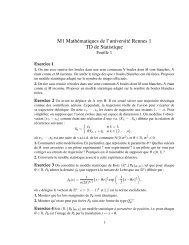
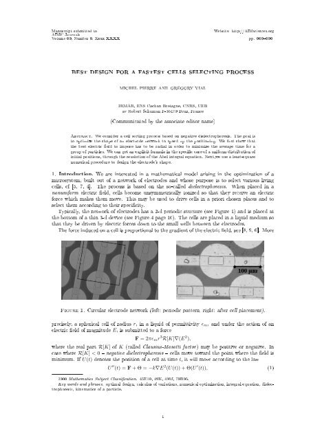
Manuscript submitted toAIMS' JournalsVolume 00, Number 0, Xxxx XXXXWebsite: http://AIMsciences.orgpp. 000000BEST DESIGN FOR A FASTEST CELLS SELECTING PROCESSMICHEL PIERRE AND GRÉGORY VIALIRMAR, ENS Cachan Bretagne, CNRS, UEBav Robert Schuman F-35170 Bruz, France(Communicated by the associate editor name)Abstract. We consider a cell sorting process based on negative dielectrophoresis. The goal isto optimize the shape of an electrode network to speed up the positioning. We rst show thatthe best electric eld to impose has to be radial in order to minimize the average time for agroup of particles. We can get an explicit formula in the specic case of a uniform distribution ofinitial positions, through the resolution of the Abel integral equation. Next,we use a least-squarenumerical procedure to design the electrode's shape.1. Introduction. We are interested in a mathematical model arising in the optimization of amicrosystem, built out of a network of electrodes and whose purpose is to select various livingcells, cf [5, 7, 4]. The process is based on the so-called dielectrophoresis. When placed in anonuniform electric eld, cells become unsymmetrically ionized so that they receive an electricforce which makes them move. This may be used to drive cells in a priori chosen places and toselect them according to their specicity.Typically, the network of electrodes has a 2-d periodic stucture (see Figure 1) and is placed atthe bottom of a thin 3-d device (see Figure 4 page 10). The cells are placed in a liquid medium sothat they be driven by electric forces down to the small wells between the electrodes.The force induced on a cell is proportional to the gradient of the electric eld, see [8, 9, 6]. MoreFigure 1. Circular electrode network (left: periodic pattern, right: after cell placement).precisely, a spherical cell of radius r, in a liquid of permittivity ɛ m , and under the action of anelectric eld of magnitude E, is submitted to a forceF = 2πɛ m r 3 R[K]∇(E 2 ),where the real part R[K] of K (called Clausius-Mosotti factor ) may be positive or negative. Incase where R[K] < 0 negative dielectrophoresis cells move toward the point where the eld isminimum. If U(t) denotes the position of a cell at time t, it will move according to the lawU ′′ (t) = F + Θ = −k∇E 2 (U(t)) + Θ(U ′ (t)), (1)2000 Mathematics Subject Classication. 45E10, 49K, 49M, 70B05.Key words and phrases. optimal design, calculus of variations, numerical optimization, integral equation, dielectrophoresis,kinematics of a particle.1

2 MICHEL PIERRE AND GRÉGORY VIALwhere k is a strictly positive constant in the case of negative dielectrophoresis, and Θ = Θ(U ′ ) takesinto account the friction forces (which are always present in the experiments under consideration).We want to control the shape of the electrodes so that the cells arrive as fast as possibleto the point where E 2 reaches its minimum. The network of electrodes is assumed to be periodic.Our strategy is as follows: we rst determine what should be the best attracting eld Eindependently of any constraint: this is essentially a control problem for a family of evolutionsystems which is mathematically interesting for itself. Then, we try to optimize the shape of theelectrodes in order to be as close as possible to this best eld. According to the law (1), the rststep consists in nding the best scalar function E 2 so that the solutions U(t) of (1), starting withzero velocity, reach the point where E 2 is minimum (say the origin) as fast as possible.A rst helpful reduction is the following (see Section 2.1 for a proof): let x 0 be a startingposition for a single particle with initial velocity zero. Given an attracting potential F = E 2 , onecan always replace it by a radial attracting eld of at most the same size, which will make theparticle reach the origin in a shorter time. It is well known that the shortest path to reach a pointin R 3 is a straight line; however, it is not always the fastest as it is well known in many situations.We prove in Section 2.1 that it is actually the case here. This is why we will mainly consider radialpotentials later on in this paper.A next question is the following: what is the best radial attracting potential to bring a particlethe fastest possible from its initial position x 0 to the origin? Actually, it is easy to see (cf.Section 2.1) that the answer will strongly depend on the starting point x 0 . Since we are moreinterested in accelerating a group of particles with a same electric eld, we will rather minimizethe average time necessary for a distributed group of particles to reach the origin. This question isanalyzed in Section 3. We prove existence and uniqueness of a best scalar eld E 2 . Surprisingly,the question leads to integral equations, one of them being well-known in the literature as the Abelintegral equation see (24).Next, we will try to design the fastest shapes of the electrodes by being as close as possibleto the previously obtained best radial attracting eld. We use a least square method and theobjective function to be minimized is an euclidian distance between the expected eld and thebest eld found before. This is analyzed numerically in Section 4.2. Towards the optimization problem.2.1. Reduction to radial elds. As stated in the introduction, we prove here that one canalways do better (= faster) with radial elds. We will essentially discuss the case when Θ ≡ 0 (nofriction). As explained in Ÿ 2 and Theorem 2.2, it is not dicult to modify the analysis so as toinclude this term. But the analysis is less technical without it and easier to read while nothing ofthe essential part is lost.We denote by | · | the euclidian norm in R N . Let F : R N \ {0} → [0, +∞) be a C 2 -function with∇F bounded in a neighborhood of the origin 0 and F (0) := lim |r|→0 F (r) = 0. Let us consider thesolution ofU ′′ (t) = −∇F (U(t)), U(0) = x 0 , U ′ (0) = 0. (2)This solution exists globally in time since: |U ′ | 2 = 2[F (x 0 ) − F (U)] ≤ 2F (x 0 ). We assume thatU(T ) = 0 for some T > 0 and we set e 0 := x 0 /|x 0 |.Theorem 2.1. There exists t 0 ∈ [0, T ), τ ∈ (t 0 , T ], G ∈ C 1 [0, |x 0 |] andu ∈ C 2 ([t 0 , τ]; R N ) such that,∀t ∈ (t 0 , τ), u ′′ (t) = −G ′ (|u(t)|)e 0 , u(t 0 ) = x 0 , u ′ (t 0 ) = 0, (3)G(0) = 0, ‖G‖ ∞ = G(|x 0 |) ≤ F (x 0 ), ‖G ′ ‖ ∞ ≤ ‖∇F ‖ ∞ . (4)u(τ) = 0, and ∀ t ∈ [t 0 , τ], |u(t)| ≤ |U(t)|. (5)Remark 1. Let us set: ∀x ∈ R N , G(x) = G(|x|). Then, for x ∈ [0, x 0 ], one has ∇G(x) = G ′ (|x|)e 0 .This theorem shows that, given x 0 , we may replace the initial potential F by a radial potential Gin such a way that the accelerated particle u(t) reaches the origin at least as fast as (and most ofthe time, faster than) the previous one U(t) and this, with a potential G bounded above by F aswell as ∇G bounded above by ∇F see (4).

FASTEST CELLS SELECTING PROCESS 3The dependence in x 0 of this new potential G is discussed below.Proof. (of Theorem 2.1) The new radial solution u(t) will be essentially constructed via the orthogonalprojection (U(t) · e 0 )e 0 of U(t) onto the direction of e 0 .We denote by τ the rst time t ∈ (0, T ] such that U(t)·e 0 = 0 (we know it exists since U(T ) = 0).To explain the idea of the proof, we rst assume that U ′′ (t) · e 0 < 0 for all t ∈ (0, τ): this meansx 0 •x 0 •u(t)•e 0•U(t)u(t 1 )•u(t 2 )•e 0• U(t 1)• U(t 2)0•0•Figure 2. Projection onto the e 0 axis (left: monotonic case, right: general case).that the attraction is directed downwards all along the trajectory (assuming e 0 denes the verticaldirection, see left picture of Figure 2). Since U ′ (0) · e 0 = 0, this also implies U ′ (t) · e 0 < 0 for allt ∈ (0, τ). Then, we set u(t) = (U(t) · e 0 )e 0 . We have, for all t ∈ [0, τ]u(0) = x 0 , |u(t)| = U(t) · e 0 , u ′′ (t) = (U ′′ (t) · e 0 )e 0 = −[∇F (U(t)) · e 0 ]e 0 . (6)Since the mapping t ∈ [0, τ] → a(t) = U(t) · e 0 = |u(t)| ∈ [0, |x 0 |] is strictly decreasing, wedenote by a −1 its inverse function (which has the same regularity as a itself). Then, we deneg : [0, |x 0 |] → [0, +∞) asg(r) = ∇F ( U(a −1 (r)) ) · e 0 .And we have, thanks to (6)∀t ∈ [0, τ], u ′′ (t) = −g(|u(t)|)e 0 .Note that g ≥ 0 due to our assumption U ′′ (t) · e 0 < 0. We now set G(r) = ∫ rg(s)ds to obtain0Theorem 2.1. By construction ‖G ′ ‖ ∞ ≤ ‖∇F ‖ ∞ and, by integration:2[G(|x 0 |) − G(|u(t)|)] = |u ′ (t)| 2 ≤ |U ′ (t)| 2 = 2[F (x 0 ) − F (U(t))]. (7)And at t = τ, since u(τ) = 0 and G(|u(τ)|) = G(0) = 0, we obtain:|u ′ (τ)| 2 = 2G(|x 0 |) ≤ |U ′ (τ)| 2 ≤ 2F (x 0 ), (8)whence the announced estimate on ‖G‖ ∞ = G(|x 0 |).Henceforth, we consider the general case where it may happen that U ′′ (t) · e 0 > 0 for somet ∈ (0, T ) (this is the case of the dashed part of the trajectory in the right picture of Figure 2),that is to say, the attraction is directed upwards at some places on the trajectory. Then, the ideais to continue going down linearly on the direction of e 0 while this happens. We introduceThen, we dene∀t ∈ [0, T ], a ′ (t) = −∫ t0[U ′′ (s) · e 0 ] − ds, a(0) = |x 0 |.t 0 = inf{t ∈ (0, T ]; U ′′ (t) · e 0 < 0}, τ = inf{t ∈ (t 0 , T ]; a(t) = 0}.Note that τ is well-dened; indeeda ′ (t) ≤∫ t0U ′′ (s) · e 0 ds = U ′ (t) · e 0 , which implies a(t) − |x 0 | ≤ U(t) · e 0 − |x 0 |.Since U(T ) · e 0 = 0, it follows that a(t) vanishes for some t ∈ (t 0 , T ].

4 MICHEL PIERRE AND GRÉGORY VIALNow, t ∈ [t 0 , τ] → a(t) ∈ [0, |x 0 |] is strictly decreasing. We denote by a −1 its inverse and wedeneK ={t ∈ [t 0 , T ]; U ′′ (t) · e 0 ≤ 0}; ∀t ∈ K, χ K (t) = 1, ∀t ∈ [t 0 , T ]\K, χ K (t) = 0, (9)∀r ∈ [0, |x 0 |], g(r) = χ K (a −1 (r)) [ ∇F ( U(a −1 (r)) ) · e 0 ]. (10)If we now set u(t) = a(t)e 0 , we have u(t 0 ) = x 0 and for all t ∈ [t 0 , τ]:u ′′ (t) = a ′′ (t)e 0 = −χ K (t)[∇F (U(t)) · e 0 ]e 0 = −g(a(t))e 0 = −g(|u(t)|)e 0 .Note that g ≥ 0 and is continuous (this only needs to be checked on the boundary of K, and it iseasy). We set G(r) = ∫ rg(s)ds and we nish as in (7)(8), checking that, here again:0G(|u(τ)|) = 0, 2G(|x 0 |) = |u ′ (τ)| ≤ |U ′ (τ) · e 0 | ≤ |U ′ (τ)| ≤ 2F (x 0 ).Remark 2. : Case of friction. Assume there is friction in the movement of the cells (which isactually always the case). In this situation, instead of (2), the evolution of each cell is given byU ′′ (t) = −∇F (U(t)) + Θ(U ′ (t)),where Θ ∈ C 1 (R N , R N ). Then Theorem 2.1 may be extended as follows:Theorem 2.2. There exists (t 0 , τ) ∈ [0, T )×(0, T ], G ∈ W 1,∞ [0, |x 0 |], h : [0, +∞) → R measurableand bounded and u ∈ C 2 ([t 0 , τ]; R N ) such that,a.e.t ∈ (t 0 , τ), u ′′ (t) = −G ′ (|u(t)|)e 0 + h(|u ′ (t)|)e 0 , u(t 0 ) = x 0 , u ′ (t 0 ) = 0, (11)G(0) = 0, ‖G ′ ‖ ∞ ≤ ‖∇F ‖ ∞ , ‖h‖ ∞ ≤ ‖Θ‖ ∞ , (12)u(τ) = 0, and ∀ t ∈ [t 0 , τ], |u(t)| ≤ |U(t)|. (13)Proof. We just indicate how to modify the proof of Theorem 2.1. We use the same function a(t)dened through the integration of −[U ′′ (t) · e 0 ] − . The mapping t ∈ [t 0 , τ] → a(t) ∈ [0, |x 0 |] isnonincreasing, where t 0 , τ are dened in the same way as in Theorem 2.1. Again, we denote itsinverse by a −1 and we dene K and g as in (9) and (10). Moreover, the mapping t → −a ′ (t) ∈[0, −a ′ (τ)] is nondecreasing. We denote by β its left-continuous inverse and we deneIt is then easy to check that∀r ′ ∈ [0, −a ′ (τ)], h(r ′ ) = χ K(β(r ′ ) ) [Θ ( U ′ (β(r ′ )) ) · e 0 ].a ′′ (t) = −g(a(t)) + h(−a ′ (t)), or u ′′ (t) = −g(|u(t)|)e 0 + h(|u ′ (t)|)e 0 .Remark 3. : Note that u ′′ remains continuous, but h may be discontinuous. Actually, if it is thecase, then τ < T . Nevertheless, we may approximate h (and also g) by more regular functions andthe associated solutions still reach the origin in time τ + ɛ < T .2.2. Best potential for a single cell. One may ask whether it is still possible to improve theradial potential G in such a way that the corresponding solution reaches the origin even faster.Let us analyze this in the case without friction. Then, it turns out that an easy expression canbe obtained for the reaching time. Let us write the solution as follows, where a(t) is a scalarfunction and G ∈ C 2 (R, R):a ′′ (t) = − 1 2 G′ (a(t)), a(0) = a 0 > 0, a ′ (0) = 0.(We added a factor 1/2 in the notation only to simplify further expressions). Since we want toaccelerate the particle towards a(·) = 0, it is better to assume that G ′ ≥ 0 (as it is the case in theG obtained in Theorem 2.1 above). This may be integrated asa ′2 (t) = G(a 0 ) − G(a(t)) or− a ′ (t) = √ G(a 0 ) − G(a(t)).

FASTEST CELLS SELECTING PROCESS 5Let us denote by τ(a 0 ) the rst time t such that a(t) = 0 (assuming it exists). Then integratingonce more the above identity, from 0 to τ(a 0 ), leads to (note that a ′ (t) ≤ 0)τ(a 0 ) =∫ τ(a0)0−a ′ ∫(t)a0√G(a0 ) − G(a(t)) dt = da√G(a0 ) − G(a) . (14)Minimizing τ(a 0 ) in this context leads to the following minimization problem: we setH = {H ∈ W 1,∞ (0, a 0 ); H ′ ≥ 0, H(0) = 0, ‖H‖ ∞ ≤ ‖G‖ ∞ , ‖H ′ ‖ ∞ ≤ ‖G ′ ‖ ∞ }.τ H (a 0 ) :=And the minimization problem becomes∫ a000da√H(a0 ) − H(a) .Find H opt ∈ H, such that τ Hopt (a 0 ) = min{τ H (a 0 ); H ∈ H}.It is straighforward to check that an optimal H is given byH m (a) = [G(a 0 ) + ‖G ′ ‖ ∞ (a − a 0 )] + .This would be a good optimal solution if we were to deal with only one particle. But we generallywant to accelerate several particles together with the same electric eld. Since the previous optimalchoice depends on a 0 , it is necessary to re-think the optimization process. This is the goal of thenext paragraph.2.3. Best average time for a group of particles. In experiments, one generally wants toaccelerate together a whole group of cells located in a region B of the origin, with the same electriceld. We will assume that B is the ball of radius 1 and centered at the origin.To take this into account, one idea is to minimize the average time taken by the whole set ofparticles to reach the origin. According to Theorem 2.1, given a potential on B, for each startingpoint x 0 , we can do better by choosing a radial modication of this potential. Therefore, it isnatural to look directly for a potential which is directed towards the origin at each point, that isto say, of the form (with e 0 = x 0 /|x 0 |)G(x 0 ) = G(x 0 )e 0 , G : B → [0, +∞),ddr G(re 0) ≥ 0, G(0) = 0. (15)The reaching time of the origin by a particle starting at x 0 = a 0 e 0 with zero initial velocity is givenby (see (14)):τ G (x 0 ) = τ G (a 0 e 0 ) =∫ a00da√G(a0 e 0 ) − G(ae 0 ) . (16)We denote by α ∈ L 1 (B) the density distribution of the particles at the beginning of the experimentwith α ≥ 0, ∫ α(x)dx = 1. We consider the minimization of the mean value of the reaching time,Bwith the weight α, namely{Find Gopt minimizing ∫ B α(x 0)τ G (x 0 )dx 0 ,among the G as in (15) and with ‖G‖ ∞ ≤ A 0 , ‖∇G‖ ∞ ≤ A 1 ,where A 0 , A 1 are a priori given bounds (with A 0 ≤ A 1 since G(0) = 0).Denoting S N−1 the unit sphere in R N , the integral to be minimized may be rewritten∫ 1∫ a0dade 0 α(a 0 e 0 )da 0 √∫S N−1 G(a0 e 0 ) − G(ae 0 ) .0Minimizing this integral is equivalent to minimize, for each e 0 , the expressionT (y) =∫ 100β(a 0 )da 0∫ a00da√y(a0 ) − y(a) , (17)where β(a 0 ) = α(a 0 e 0 ), y(a) = G(ae 0 ). This is the purpose of next Section.

6 MICHEL PIERRE AND GRÉGORY VIAL3. Best potential; the Abel integral equation. As suggested in the previous section, weconsider the reaching time functionalT (y) =∫ 10β(a 0 )da 0∫ a0where β ∈ L 1 (0, 1), β ≥ 0 and y ∈ M where0da√ ≤ +∞, (18)y(a0 ) − y(a)M={y : [0, 1] → [0, 1] nondecreasing, y(0):= lima→0y(a)=0, y(1):= lima→1y(a)=1}.The choice of y(1) = 1 is only a normalization (more generally, we would work with y/‖y‖ ∞ ). Notethat a function y ∈ M is not well dened at its discontinuity points. But they form an at mostcountable set so that the integral T (y) is well dened.We consider the minimization problemWe have a rst result.y ∗ ∈ M, T (y ∗ ) = min{T (y); y ∈ M}. (19)Proposition 1. There exists y ∗ solution of (19). When β > 0 a.e. on a neighborhood of 1, thenit is unique (more precisely, two solutions are equal except for their values at their discontinuitypoints). If β > 0 a.e., then y ∗ is strictly increasing.Proof. Note that if y(x) = x, then T (y) = ∫ 10 2β(a 0) √ a 0 da 0 < +∞, so that I = inf{T (y); y ∈M} < +∞.Let (y n ) n≥1 ∈ M be such that T (y n ) converges to I . Since the y n 's are nondecreasing andbounded, we may assume, up to a subsequence, that they converge a.e. to a nondecreasing functiony ∗ : [0, 1] → [0, 1]. By Fatou's Lemma, we have T (y ∗ ) ≤ I.It remains to check the boundary conditions y ∗ (0) = 0, y ∗ (1) = 1: it will follow that y ∗ ∈ M andis a minimum for (19). First, y ∗ cannot be a constant function since it would make T (y ∗ ) = +∞.Next, we notice that, if z = [y ∗ − y ∗ (0)]/[y ∗ (1) − y ∗ (0)], we have z ∈ M andI ≤ T (z) = √ y ∗ (1) − y ∗ (0) T (y ∗ ) = √ y ∗ (1) − y ∗ (0) I.This proves y ∗ (1) − y ∗ (0) = 1, whence the expected boundary conditions.For the uniqueness, let us work with the representation of y ∗ which is right-continuous on[0, 1). We remark that y → T (y) is convex for all β, and even strictly convex if β > 0 a.e. ona neighborhood of 1, as one can easily check using the strict convexity of the function r → √ 1 r:whence the uniqueness of the minimum of T (·).Assume now β > 0 a.e.: if y ∗ was constant on some interval, we would have T (y ∗ ) = +∞ whichis a contradiction; thus, y ∗ is strictly increasing.Computation of the optimal solution y ∗ : It is elementary to write down an optimizationalgorithm to compute y ∗ (remember that the fonctional y → T (y) is convex). We used here axed step gradient method based on a linear discretization. Figure 3 shows the results obtained forseveral values of β. The only numerical point to worry about is the fact that y ∗ may be constant(or almost constant) at some places. For instance, we may check thatIndeed, we may then writeT (y) =∫ 1α(β = 0 on [0, α)β(a 0 )da 0[ ∫ α0)=⇒(y ∗ = 0 on [0, α]). (20)∫ ]daa0√y(a0 ) − y(a) + da√ .y(a0 ) − y(a)Obviously, given y, if one replaces it by ỹ which equal to zero on [0, α] and equal to y on [α, 1], wehave T (ỹ) ≤ T (y).We denote by T β the reaching time functional associated with a given distribution β, and by y ∗ βthe corresponding optimal solution. In Table 1, we compare the times T β (y) for various β and y.For β = β 1 ≡ 1, the computations are explicit, while they result from a numerical method with 50discretization points otherwise.Analysis of y ∗ : It turns out that the analysis of the optimal solution y ∗ is not so easy. Inparticular, we do not know exactly its regularity. We are able to write down the Euler-Lagrangeα

FASTEST CELLS SELECTING PROCESS 7y ⋆ (a)1β(x) = 1β(x) = xβ(x) = 2χ [0.5,1] (x)β(x) = (0.7) −1 (1 − χ [0.2,0.5] (x))0 0.51aFigure 3. Optimal solutions y∗ obtained for dierent β.y y ∗ β 1x ↦→ x x ↦→ x 2T β1 (y)π 3/22 √ 2Γ(3/4) 2 ≃ 1.31 43 ≃ 1.33 π2 ≃ 1.57y y ∗ β 2x ↦→ x y β1T β2 (y) 1.43 1.72 1.67y y ∗ β 3x ↦→ x y β1T β3 (y) 1.36 1.40 1.39Table 1. Reaching times for β 1 ≡ 1, β 2 = 2χ [0.5,1] and β 3 = (0.7) −1 (1 − χ [0.2,0.5] ).equation (or optimality condition) in general (see Proposition 2 below). But, it is not easy toexploit it, even in the case β ≡ 1. Actually, in this specic case, the optimality condition can bereformulated in a dierent way: this is done in Proposition 3. Surprisingly, this leads to an integralequation, with unknown function (or more precisely measure) µ(a) = d da [y∗ ] −1 (a), which is ratherwell known and widely studied in the literature (sometimes called Abel equation, see for instancethe paper [2] or the books [1, Chap. 7], [10] on this subject). Using these results, we deduce anexplicit expression for y ∗ in this case (which allows to conrm the computations above). Theseproperties of y ∗ are summarized in the next two propositions.Proposition 2. Let y ∗ be an optimal solution as in Proposition 1 and let ν = ddx y∗ (which is anonnegative measure of mass 1). Thenν − a.e. ξ, H(ξ) :=∫ ξ0da∫ 1ξβ(a 0 )[y ∗ (a 0 ) − y ∗ (a)] −3/2 da 0 = T (y ∗ ). (21)

8 MICHEL PIERRE AND GRÉGORY VIALProposition 3. Assume β ≡ 1. Then, the optimality condition also reads∀x ∈ (0, 1),∫ 10da√|x − y∗ (a)| = 2T (y∗ ) =where µ ∗ = d dt [y∗ ] −1 . Its unique solution is given by[∫ 1−1µ ∗ (t) = k [t(1 − t)] −1/4 dt where k = [t(1 − t)] dt] −1/4 =0∫ 10dµ ∗ (t)√|x − t|, (22)√ π2 Γ ( )3 2. (23)4Remark 4. By Proposition 1, we know that y ∗ is strictly increasing. As a consequence, its inversefunction z ∗ (t) = [y ∗ ] −1 (t) is continuous, nondecreasing on [0, 1]. Its derivative µ ∗ = d dt z∗ is anonnegative measure without atoms. The above theorem claims that µ ∗ = ˆkλ where λ is theunique solution of the following so-called Abel integral equation with constant limits of integrationamong the nonnegative measures:∀x ∈ [0, 1],∫ 10dλ(t)√|x − t|= 1. (24)The constant ˆk is adjusted so that ∫ 10 dµ∗ = 1. It turns out that the solution of (24) is explicitelyknown as being t → [π √ 2] −1 [t(1 − t)] −1/4 . For convenience, this is proved completely below, butthis exact expression was essentially guessed from various results in [2, 3, 1, 10]. It follows alsothat T (y ∗ ) =π 3/22 √ 2Γ(3/4) 2 .Proof. (of Proposition 2) It is a priori not clear that H(ξ) is nite for all ξ. We rst notice that itis the increasing limit as η decreases to 0 ofη ∈ (0, 1) → H η (ξ) =∫ ξ0da∫ 1ξβ(a 0 )[(y ∗ (a 0 ) − y ∗ (a)) + η] −3/2 da 0 .In particular, it is lower semi-continuous on [0, 1] since H η is obviously continuous.∫ We will use several times the following identity: let λ be a nonnegative measure on (0, 1) withdλ = 1 and let Λ be the right-continuous increasing function such that(0,1)∫∀0 ≤ a ≤ a 0 ≤ 1, Λ(a 0 ) − Λ(a) = dλ.Then, by Fubini' theorem (note that all functions involved are nonnegative)∫∫ 1 ∫ a0Λ(a 0 ) − Λ(a)H(ξ) dλ(ξ) = da 0 β(a 0 )da ≤ +∞. (25)[y ∗ (a 0 ) − y ∗ (a)]3/2(0,1)00If ν = d da y∗ , then applying this with λ = ν, and using the denition (18) of T , we obtain∫H(ξ) dν(ξ) = T (y ∗ ). (26)(0,1)This proves at least that H is nite ν-a.e..Let now ψ ∈ C [0, 1] with ψ ≥ 0 and ϕ(x) = ∫ x0 ψ(t)dt. Then, for t > 0, the function (y∗ +tϕ)/(1 + tϕ(1)) ∈ M and by minimality of y ∗ :( yT (y ∗ ∗ )+ tϕ) ≤ T= √ 1 + tϕ(1) T (y ∗ + tϕ). (27)1 + tϕ(1)Set c = y ∗ (a 0 ) − y ∗ (a) ≥ 0 and d = ϕ(a 0 ) − ϕ(a) ≥ 0. We haveT (y ∗ ) − T (y ∗ + tϕ) =∫ 10β(a 0 )da 0∫ a00(a,a 0]t d da√c(c + td)[√ c +√c + td], (28)and by (27), this is bounded above by T (y ∗ + tϕ)[ √ 1 + tϕ(1) − 1]. Dividing this inequality byt > 0 and letting t tend to zero yield:∫ 10β(a 0 )da 0∫ a00d dac 3/2 ≤ ϕ(1)T (y∗ ). (29)

FASTEST CELLS SELECTING PROCESS 9In particular, the integral on the left hand-side is nite. Plugging d = ∫ a 0ψ(ξ)dξ, and using (25),athis may also be written∫ 1∫ 1ψ(ξ)H(ξ)dξ ≤ ϕ(1)T (y ∗ ) = ψ(ξ)T (y ∗ )dξ.0By arbitrarity of ψ, this implies: H(ξ) ≤ T (y ∗ ) a.e. ξ ∈ (0, 1). Since H is lower semi-continuous,the set {ξ ∈ (0, 1); H(ξ) > T (y ∗ )} is open; being of Lebesgue-measure zero, it is empty. Therefore,H(ξ) ≤ T (y ∗ ) for all ξ ∈ (0, 1). Combined with (26), this implies the expected equality (21).Remark 5. : Since we do not have any a priori regularity for y ∗ , we cannot say anything aboutthe structure of the measure ν. It may a priori contain singular parts, orthogonal to the Lebesguemeasure, or Dirac masses, since even the continuity of y ∗ is not clear in general.Proof. (of Proposition 3) Let µ(t) = [t(1 − t)] −1/4 . Let us prove successively that[∫ ]1dµ(t)x ∈ [0, 1] → √ is constant , (30)|x − t|and, if z(t) = k ∫ t0To prove (30), we set0dµ(s) where k is such that z(1) = 1, then for y = z−1ξ ∈ (0, 1) →∫ ξ0da∫ 1ξI(x) :=0[y(a 0 ) − y(a)] −3/2 da 0 = constant. (31)and we make the change of variable t = (1 + cos ϕ)/2, ϕ ∈ [0, π]; then∫ π()sin ϕI(x) = J(θ) = Fdϕ,| cos θ − cos ϕ|∫ 1with cos θ = 2x − 1 (θ ∈ [0, π]), and F (r) = √ r. We write∫ θ() ∫sin ϕπ(J(θ) = Fdϕ + Fcos ϕ − cos θ000[t(1 − t)] −1/4 dt√|x − t|, (32)θsin ψcos θ − cos ψ)dψ,and we make the following one-to-one changes of variables, respectively in each integralsin ϕu =cos ϕ − cos θ , u = sin ψcos θ − cos ψ . (33)This givesJ(θ) =∫ +∞0F (u)ϕ ′ (u)du −∫ +∞But, the two functions ϕ(u), ψ(u) dened in (33) are such that( )1 cos ϕ − cos ψ ϕ − ψ=u sin ϕ + sin ψ = − tan ,20F (u)ψ ′ (u)du. (34)so that ϕ ′ (u) − ψ ′ (u) = 2[1 + u 2 ] −1 is independent of θ. It follows from the expression (34) thatJ(θ) is also independent of θ.Let us now prove (31). By making the change of variable t = y(a) ⇔ a = z(t), we have∫ 10k dµ(t)√|x − t|=∫ 10da√|x − y(a)|.We will compare the derivative of this function with the derivative of the function involved in (31).But, we rst regularize them as follows: for η > 0, we denoteThenG η (x) =∫ 10da√|x − y(a)| + η, H η (ξ) =2G ′ η(x) =∫ 10∫ ξ0da∫ 1−sign(x − y(a))da[|x − y(a)| + η] 3/2 ,ξda 0[y(a 0 ) − y(a) + η] 3/2 .

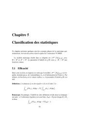
10 MICHEL PIERRE AND GRÉGORY VIALH ′ η(ξ) =∫ 1ξ∫da ξ0[y(a 0 ) − y(ξ) + η] − da3/2 [y(ξ) − y(a) + η] . 3/2We have 2G ′ η(y(ξ)) = H ′ η(ξ), which implies that for all ψ ∈ C ∞ 0 (0, 1):−∫ 10ψ ′ (ξ)H η (ξ)dξ =∫ 102G ′ η(y(ξ))ψ(ξ)dξ =0∫ 102G ′ η(x)ψ(z(x))z ′ (x)dx. (35)As η decreases to zero, the function G η increases to the function G 0 which is constant by (30):therefore, its derivative converges to zero in the sense of distributions on (0, 1). We deduce thatthe integrals in (35) tend to zero (note that ψ(z(·))z ′ (·) ∈ C0 ∞ (0, 1)): this says that H η ′ convergesto 0 in the sense of distributions and this implies (31).To end the proof of Proposition 3, note that the constant in (31) is necessarily equal to T (y)since, ∫ 1 d0 dξ y(ξ)H 0(ξ)dξ = T (y) (see the computations (25)(26) where we replace y ∗ by y). Thenit follows that y satises the rst order optimality condition of Proposition 2. By strict convexityof y ∈ M → T (y), we deduce that y = y ∗ . Indeed, according to the convexity of T (·) and to thecomputations (28), (29), we may write for all y ∈ M:T (y ∗ ) − T (y) ≥ d dt | t=0T ((1 − t)y + ty ∗ ) =∫ 10da 0∫ a00da (y∗ − y)(a 0 ) − (y ∗ − y)(a)[y(a 0 ) − y(a)] 3/2 ,and by (25)∫ 1∫T (y ∗ d1d) − T (y) ≥0 dξ [y∗ − y](ξ)H 0 (ξ)dξ = T (y)0 dξ [y∗ − y](ξ)dξ = 0.Whence T (y) = T (y ∗ ).Note also that the constant in (30) is 2T (y), since after setting x = y(a 0 ) and integrating withrespect to a 0 , we see that this constant is equal to:∫∫da 0 da1 ∫ a0∫√(0,1) 2 |y(a0 ) − y(a)| = da1 ∫ 1da 0 √0 y(a0 ) − y(a) + dada 0 √ = 2T (y).0 y(a) − y(a0 )0a 04. Numerical shape optimization of the electrodes. The microsystem we aim at designingis composed of a periodic network of interdigited electrodes, see Figure 1. We will optimize theshape of the electrodes in the box of Figure 4, the whole device being deduced by periodicity. Asdepicted, the opposite electrodes have the same polarity. Furthermore, the four electrodes havethe same shape to enforce symmetry and ensure that the eld E vanishes at the center G of thebottom. Of course, the dielectrophoretic potential E 2 = ‖E‖ 2 is minimal at G, and we expect thecells to move towards this point.Our numerical strategy consists in nding the best electrodes to produce a eld as close aspossible to the optimal eld obtained in section 3. Since the methods we used are quite standard,we will only give a brief description and show the simulation results.zx+−G•−+yFigure 4. Periodic pattern for computations.

FASTEST CELLS SELECTING PROCESS 114.1. Computation of the electric eld for a given shape. Due to the periodicity conditionson the lateral sides of the box, we use a description of the unknowns in terms of Fourier series.Precisely, the electric potential V is written asV (x, y, z) = ∑V k,l (z)e iω(kx+ly) , (36)k,l∈Zwith ω = 2π/L where L is the common edge-length in the x and y directions.The electrodes E ± are supposed to be innitely thin and are integrated through boundaryconditions on z = 0. Besides, it is not clear which boundary condition has to be imposed onthe top side of the box, and it is more natural to consider a semi-innite beam with evanescentcondition at z → +∞. Altogether, the electric potential solves the following Laplace problem:⎧−∆V (x, y, z) = 0 for (x, y, z) ∈ [0, L] × [0, L] × [0, +∞),⎪⎨ V (x, y, 0) = ±V 0 for (x, y) ∈ E ± ,(37)∂ z V (x, y, 0) = 0 for (x, y) /∈ E ± ,⎪⎩V (x, y, z) → 0 as z → +∞.The coecients V k,l (z) are given byV k,l (z) = V k,l (0)e −ωz√ k 2 +l 2 ,so that problem (37) reduces to the following linear equation on the V k,l (0):∑V k,l (0)e iω(kx+ly) = ±V 0 for (x, y) ∈ E ± ,k,l∈Z∑k,l∈ZV k,l (0) √ k 2 + l 2 e iω(kx+ly) = 0 for (x, y) /∈ E ± .If the discretization incorporates N Fourier frequencies, a collocation method leads to a full N × Nlinear system. The electric potential V is reconstructed via inverse fast Fourier transform, as wellas the electric eldE = −∇V.4.2. Least square optimization. The optimal electric eld being determined according to Section3, we now design the electrodes to produce the closest eld in a least square sense. Asmentioned above, we force the electrodes to be identical (another symmetry axis is also imposed inthe computations below). We start from circular shapes which were already considered to be thebest shapes from an experimental point of view, among those considered in [4]. Then, we apply adescent method for the optimization criterion:∫Find E minimizing ‖E − E ∗ ‖ 2 = (E − E ∗ ) 2 (x, y)dxdy, (38)where the target eld E ∗ is given in Section 3 and where Ω is a region of interest around the originin the horizontal section z = 1/30 which corresponds to experimental initial positions of the cells(note that choosing the whole box for Ω would not be very relevant since the eld produced byplanar electrodes does certainly have a completely non-radial structure).The electrodes are represented by a spline interpolation of control points. Figure 5 shows theelectrodes obtained with 5 such points after the optimization process (the procedure consists ina periodic relaxation among boundary deformations of the electrodes along the normal vector ateach control point).We may compare the average time of a particle to reach the minimum of the eld for the twosituations of Figure 5. A Monte-Carlo method coupled with the numerical resolution of the ordinarydierential equation (2) attests a gain of about 20% with respect to the best knows shapes see [4].Finally, let us mention that we also applied our optimization algorithm by replacing the leastsquareobjective (38) by the average numerical reaching time. The obtained electrodes are similarto those of Figure 5, with comparable optimal reaching times.Acknowledgements : We thank Bruno LePioue and Marie Frénéa-Robin for having suggestedthis nice problem, and Martin Costabel for fruitful discussions around it.Ω

12 MICHEL PIERRE AND GRÉGORY VIAL•• ••• ••• ••Figure 5. Initial circular electrodes (left) and optimized electrodes (right).REFERENCES[1] A. V. Bitsadze. Integral equations of rst kind, volume 7 of Series on Soviet and East European Mathematics.World Scientic Publishing Co. Inc., River Edge, NJ 1995.[2] T. Carleman. Über die Abelsche Integralgleichung mit konstanten Integrationsgrenzen. Math. Z. 15(1) (1922)111120.[3] G. I. Eskin. Boundary value problems for elliptic pseudodierential equations, volume 52 of Translations ofMathematical Monographs. American Mathematical Society, Providence, R.I. 1981. Translated from the Russianby S. Smith.[4] M. Frénéa, S. P. Faure, B. L. Pioufle, P. Coquet, H. Fujita. Positioning living cells on a high-densityelectrode array by negative dielectrophoresis. Materials Science and Engineering: C 23(5) (2003) 597603.[5] Y. Huang, R. Pethig. Electrode design for negative dielectrophoresis. Measurement Science and Technology2(12) (1991) 11421146.[6] T. Jones. Electromechanics of Particles. Cambridge University Press, Cambridge 1995.[7] H. Morgan, M. P. Hughes, N. G. Green. Separation of submicron bioparticles by dielectrophoresis. Biophysicaljournal 77(1) (1999) 516525.[8] H. A. Pohl. The motion and precipitation of suspensoids in divergent electric elds. Journal of Applied Physics22(7) (1951) 869871.[9] H. A. Pohl. Dielectrophoresis. Cambridge University Press, Cambridge 1978.[10] A. D. Polyanin, A. V. Manzhirov. Handbook of integral equations. Chapman & Hall/CRC, Boca Raton,FL, second edition 2008.E-mail address: michel.pierre@bretagne.ens-cachan.frE-mail address: gregory.vial@bretagne.ens-cachan.fr