best design for a fastest cells selecting process - ENS de Cachan ...

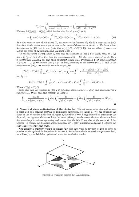
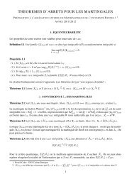
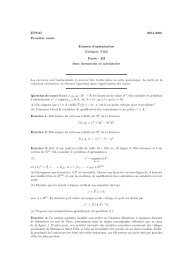
10 MICHEL PIERRE AND GRÉGORY VIALH ′ η(ξ) =∫ 1ξ∫da ξ0[y(a 0 ) − y(ξ) + η] − da3/2 [y(ξ) − y(a) + η] . 3/2We have 2G ′ η(y(ξ)) = H ′ η(ξ), which implies that for all ψ ∈ C ∞ 0 (0, 1):−∫ 10ψ ′ (ξ)H η (ξ)dξ =∫ 102G ′ η(y(ξ))ψ(ξ)dξ =0∫ 102G ′ η(x)ψ(z(x))z ′ (x)dx. (35)As η decreases to zero, the function G η increases to the function G 0 which is constant by (30):therefore, its derivative converges to zero in the sense of distributions on (0, 1). We deduce thatthe integrals in (35) tend to zero (note that ψ(z(·))z ′ (·) ∈ C0 ∞ (0, 1)): this says that H η ′ convergesto 0 in the sense of distributions and this implies (31).To end the proof of Proposition 3, note that the constant in (31) is necessarily equal to T (y)since, ∫ 1 d0 dξ y(ξ)H 0(ξ)dξ = T (y) (see the computations (25)(26) where we replace y ∗ by y). Thenit follows that y satises the rst order optimality condition of Proposition 2. By strict convexityof y ∈ M → T (y), we deduce that y = y ∗ . Indeed, according to the convexity of T (·) and to thecomputations (28), (29), we may write for all y ∈ M:T (y ∗ ) − T (y) ≥ d dt | t=0T ((1 − t)y + ty ∗ ) =∫ 10da 0∫ a00da (y∗ − y)(a 0 ) − (y ∗ − y)(a)[y(a 0 ) − y(a)] 3/2 ,and by (25)∫ 1∫T (y ∗ d1d) − T (y) ≥0 dξ [y∗ − y](ξ)H 0 (ξ)dξ = T (y)0 dξ [y∗ − y](ξ)dξ = 0.Whence T (y) = T (y ∗ ).Note also that the constant in (30) is 2T (y), since after setting x = y(a 0 ) and integrating withrespect to a 0 , we see that this constant is equal to:∫∫da 0 da1 ∫ a0∫√(0,1) 2 |y(a0 ) − y(a)| = da1 ∫ 1da 0 √0 y(a0 ) − y(a) + dada 0 √ = 2T (y).0 y(a) − y(a0 )0a 04. Numerical shape optimization of the electrodes. The microsystem we aim at designingis composed of a periodic network of interdigited electrodes, see Figure 1. We will optimize theshape of the electrodes in the box of Figure 4, the whole device being deduced by periodicity. Asdepicted, the opposite electrodes have the same polarity. Furthermore, the four electrodes havethe same shape to enforce symmetry and ensure that the eld E vanishes at the center G of thebottom. Of course, the dielectrophoretic potential E 2 = ‖E‖ 2 is minimal at G, and we expect thecells to move towards this point.Our numerical strategy consists in nding the best electrodes to produce a eld as close aspossible to the optimal eld obtained in section 3. Since the methods we used are quite standard,we will only give a brief description and show the simulation results.zx+−G•−+yFigure 4. Periodic pattern for computations.