best design for a fastest cells selecting process - ENS de Cachan ...

More documents

Recommendations

Info

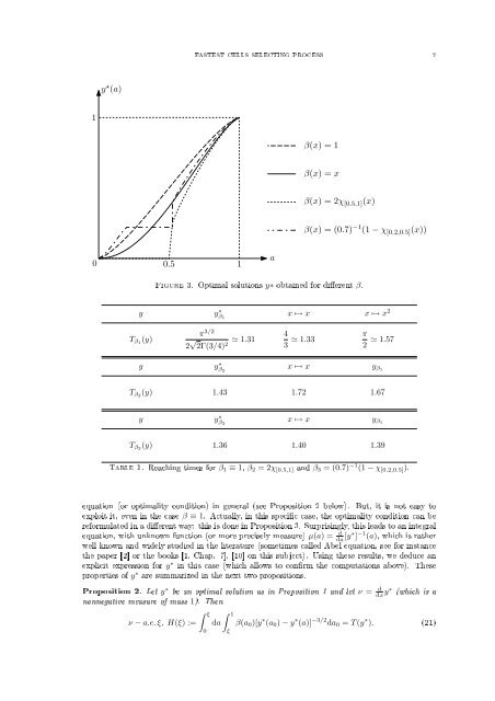
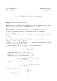
6 MICHEL PIERRE AND GRÉGORY VIAL3. Best potential; the Abel integral equation. As suggested in the previous section, weconsider the reaching time functionalT (y) =∫ 10β(a 0 )da 0∫ a0where β ∈ L 1 (0, 1), β ≥ 0 and y ∈ M where0da√ ≤ +∞, (18)y(a0 ) − y(a)M={y : [0, 1] → [0, 1] nondecreasing, y(0):= lima→0y(a)=0, y(1):= lima→1y(a)=1}.The choice of y(1) = 1 is only a normalization (more generally, we would work with y/‖y‖ ∞ ). Notethat a function y ∈ M is not well dened at its discontinuity points. But they form an at mostcountable set so that the integral T (y) is well dened.We consider the minimization problemWe have a rst result.y ∗ ∈ M, T (y ∗ ) = min{T (y); y ∈ M}. (19)Proposition 1. There exists y ∗ solution of (19). When β > 0 a.e. on a neighborhood of 1, thenit is unique (more precisely, two solutions are equal except for their values at their discontinuitypoints). If β > 0 a.e., then y ∗ is strictly increasing.Proof. Note that if y(x) = x, then T (y) = ∫ 10 2β(a 0) √ a 0 da 0 < +∞, so that I = inf{T (y); y ∈M} < +∞.Let (y n ) n≥1 ∈ M be such that T (y n ) converges to I . Since the y n 's are nondecreasing andbounded, we may assume, up to a subsequence, that they converge a.e. to a nondecreasing functiony ∗ : [0, 1] → [0, 1]. By Fatou's Lemma, we have T (y ∗ ) ≤ I.It remains to check the boundary conditions y ∗ (0) = 0, y ∗ (1) = 1: it will follow that y ∗ ∈ M andis a minimum for (19). First, y ∗ cannot be a constant function since it would make T (y ∗ ) = +∞.Next, we notice that, if z = [y ∗ − y ∗ (0)]/[y ∗ (1) − y ∗ (0)], we have z ∈ M andI ≤ T (z) = √ y ∗ (1) − y ∗ (0) T (y ∗ ) = √ y ∗ (1) − y ∗ (0) I.This proves y ∗ (1) − y ∗ (0) = 1, whence the expected boundary conditions.For the uniqueness, let us work with the representation of y ∗ which is right-continuous on[0, 1). We remark that y → T (y) is convex for all β, and even strictly convex if β > 0 a.e. ona neighborhood of 1, as one can easily check using the strict convexity of the function r → √ 1 r:whence the uniqueness of the minimum of T (·).Assume now β > 0 a.e.: if y ∗ was constant on some interval, we would have T (y ∗ ) = +∞ whichis a contradiction; thus, y ∗ is strictly increasing.Computation of the optimal solution y ∗ : It is elementary to write down an optimizationalgorithm to compute y ∗ (remember that the fonctional y → T (y) is convex). We used here axed step gradient method based on a linear discretization. Figure 3 shows the results obtained forseveral values of β. The only numerical point to worry about is the fact that y ∗ may be constant(or almost constant) at some places. For instance, we may check thatIndeed, we may then writeT (y) =∫ 1α(β = 0 on [0, α)β(a 0 )da 0[ ∫ α0)=⇒(y ∗ = 0 on [0, α]). (20)∫ ]daa0√y(a0 ) − y(a) + da√ .y(a0 ) − y(a)Obviously, given y, if one replaces it by ỹ which equal to zero on [0, α] and equal to y on [α, 1], wehave T (ỹ) ≤ T (y).We denote by T β the reaching time functional associated with a given distribution β, and by y ∗ βthe corresponding optimal solution. In Table 1, we compare the times T β (y) for various β and y.For β = β 1 ≡ 1, the computations are explicit, while they result from a numerical method with 50discretization points otherwise.Analysis of y ∗ : It turns out that the analysis of the optimal solution y ∗ is not so easy. Inparticular, we do not know exactly its regularity. We are able to write down the Euler-Lagrangeα
FASTEST CELLS SELECTING PROCESS 7y ⋆ (a)1β(x) = 1β(x) = xβ(x) = 2χ [0.5,1] (x)β(x) = (0.7) −1 (1 − χ [0.2,0.5] (x))0 0.51aFigure 3. Optimal solutions y∗ obtained for dierent β.y y ∗ β 1x ↦→ x x ↦→ x 2T β1 (y)π 3/22 √ 2Γ(3/4) 2 ≃ 1.31 43 ≃ 1.33 π2 ≃ 1.57y y ∗ β 2x ↦→ x y β1T β2 (y) 1.43 1.72 1.67y y ∗ β 3x ↦→ x y β1T β3 (y) 1.36 1.40 1.39Table 1. Reaching times for β 1 ≡ 1, β 2 = 2χ [0.5,1] and β 3 = (0.7) −1 (1 − χ [0.2,0.5] ).equation (or optimality condition) in general (see Proposition 2 below). But, it is not easy toexploit it, even in the case β ≡ 1. Actually, in this specic case, the optimality condition can bereformulated in a dierent way: this is done in Proposition 3. Surprisingly, this leads to an integralequation, with unknown function (or more precisely measure) µ(a) = d da [y∗ ] −1 (a), which is ratherwell known and widely studied in the literature (sometimes called Abel equation, see for instancethe paper [2] or the books [1, Chap. 7], [10] on this subject). Using these results, we deduce anexplicit expression for y ∗ in this case (which allows to conrm the computations above). Theseproperties of y ∗ are summarized in the next two propositions.Proposition 2. Let y ∗ be an optimal solution as in Proposition 1 and let ν = ddx y∗ (which is anonnegative measure of mass 1). Thenν − a.e. ξ, H(ξ) :=∫ ξ0da∫ 1ξβ(a 0 )[y ∗ (a 0 ) − y ∗ (a)] −3/2 da 0 = T (y ∗ ). (21)
Page 1 and 2: Manuscript submitted toAIMS' Journa
Page 3 and 4: FASTEST CELLS SELECTING PROCESS 3Th
Page 5: FASTEST CELLS SELECTING PROCESS 5Le
Page 9 and 10: FASTEST CELLS SELECTING PROCESS 9In
Page 11 and 12: FASTEST CELLS SELECTING PROCESS 114

best design for a fastest cells selecting process - ENS de Cachan ...

You also want an ePaper? Increase the reach of your titles

Delete template?

Save as template?