best design for a fastest cells selecting process - ENS de Cachan ...

More documents

Recommendations

Info

2 MICHEL PIERRE AND GRÉGORY VIALwhere k is a strictly positive constant in the case of negative dielectrophoresis, and Θ = Θ(U ′ ) takesinto account the friction forces (which are always present in the experiments under consideration).We want to control the shape of the electrodes so that the cells arrive as fast as possibleto the point where E 2 reaches its minimum. The network of electrodes is assumed to be periodic.Our strategy is as follows: we rst determine what should be the best attracting eld Eindependently of any constraint: this is essentially a control problem for a family of evolutionsystems which is mathematically interesting for itself. Then, we try to optimize the shape of theelectrodes in order to be as close as possible to this best eld. According to the law (1), the rststep consists in nding the best scalar function E 2 so that the solutions U(t) of (1), starting withzero velocity, reach the point where E 2 is minimum (say the origin) as fast as possible.A rst helpful reduction is the following (see Section 2.1 for a proof): let x 0 be a startingposition for a single particle with initial velocity zero. Given an attracting potential F = E 2 , onecan always replace it by a radial attracting eld of at most the same size, which will make theparticle reach the origin in a shorter time. It is well known that the shortest path to reach a pointin R 3 is a straight line; however, it is not always the fastest as it is well known in many situations.We prove in Section 2.1 that it is actually the case here. This is why we will mainly consider radialpotentials later on in this paper.A next question is the following: what is the best radial attracting potential to bring a particlethe fastest possible from its initial position x 0 to the origin? Actually, it is easy to see (cf.Section 2.1) that the answer will strongly depend on the starting point x 0 . Since we are moreinterested in accelerating a group of particles with a same electric eld, we will rather minimizethe average time necessary for a distributed group of particles to reach the origin. This question isanalyzed in Section 3. We prove existence and uniqueness of a best scalar eld E 2 . Surprisingly,the question leads to integral equations, one of them being well-known in the literature as the Abelintegral equation see (24).Next, we will try to design the fastest shapes of the electrodes by being as close as possibleto the previously obtained best radial attracting eld. We use a least square method and theobjective function to be minimized is an euclidian distance between the expected eld and thebest eld found before. This is analyzed numerically in Section 4.2. Towards the optimization problem.2.1. Reduction to radial elds. As stated in the introduction, we prove here that one canalways do better (= faster) with radial elds. We will essentially discuss the case when Θ ≡ 0 (nofriction). As explained in Ÿ 2 and Theorem 2.2, it is not dicult to modify the analysis so as toinclude this term. But the analysis is less technical without it and easier to read while nothing ofthe essential part is lost.We denote by | · | the euclidian norm in R N . Let F : R N \ {0} → [0, +∞) be a C 2 -function with∇F bounded in a neighborhood of the origin 0 and F (0) := lim |r|→0 F (r) = 0. Let us consider thesolution ofU ′′ (t) = −∇F (U(t)), U(0) = x 0 , U ′ (0) = 0. (2)This solution exists globally in time since: |U ′ | 2 = 2[F (x 0 ) − F (U)] ≤ 2F (x 0 ). We assume thatU(T ) = 0 for some T > 0 and we set e 0 := x 0 /|x 0 |.Theorem 2.1. There exists t 0 ∈ [0, T ), τ ∈ (t 0 , T ], G ∈ C 1 [0, |x 0 |] andu ∈ C 2 ([t 0 , τ]; R N ) such that,∀t ∈ (t 0 , τ), u ′′ (t) = −G ′ (|u(t)|)e 0 , u(t 0 ) = x 0 , u ′ (t 0 ) = 0, (3)G(0) = 0, ‖G‖ ∞ = G(|x 0 |) ≤ F (x 0 ), ‖G ′ ‖ ∞ ≤ ‖∇F ‖ ∞ . (4)u(τ) = 0, and ∀ t ∈ [t 0 , τ], |u(t)| ≤ |U(t)|. (5)Remark 1. Let us set: ∀x ∈ R N , G(x) = G(|x|). Then, for x ∈ [0, x 0 ], one has ∇G(x) = G ′ (|x|)e 0 .This theorem shows that, given x 0 , we may replace the initial potential F by a radial potential Gin such a way that the accelerated particle u(t) reaches the origin at least as fast as (and most ofthe time, faster than) the previous one U(t) and this, with a potential G bounded above by F aswell as ∇G bounded above by ∇F see (4).
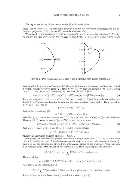
FASTEST CELLS SELECTING PROCESS 3The dependence in x 0 of this new potential G is discussed below.Proof. (of Theorem 2.1) The new radial solution u(t) will be essentially constructed via the orthogonalprojection (U(t) · e 0 )e 0 of U(t) onto the direction of e 0 .We denote by τ the rst time t ∈ (0, T ] such that U(t)·e 0 = 0 (we know it exists since U(T ) = 0).To explain the idea of the proof, we rst assume that U ′′ (t) · e 0 < 0 for all t ∈ (0, τ): this meansx 0 •x 0 •u(t)•e 0•U(t)u(t 1 )•u(t 2 )•e 0• U(t 1)• U(t 2)0•0•Figure 2. Projection onto the e 0 axis (left: monotonic case, right: general case).that the attraction is directed downwards all along the trajectory (assuming e 0 denes the verticaldirection, see left picture of Figure 2). Since U ′ (0) · e 0 = 0, this also implies U ′ (t) · e 0 < 0 for allt ∈ (0, τ). Then, we set u(t) = (U(t) · e 0 )e 0 . We have, for all t ∈ [0, τ]u(0) = x 0 , |u(t)| = U(t) · e 0 , u ′′ (t) = (U ′′ (t) · e 0 )e 0 = −[∇F (U(t)) · e 0 ]e 0 . (6)Since the mapping t ∈ [0, τ] → a(t) = U(t) · e 0 = |u(t)| ∈ [0, |x 0 |] is strictly decreasing, wedenote by a −1 its inverse function (which has the same regularity as a itself). Then, we deneg : [0, |x 0 |] → [0, +∞) asg(r) = ∇F ( U(a −1 (r)) ) · e 0 .And we have, thanks to (6)∀t ∈ [0, τ], u ′′ (t) = −g(|u(t)|)e 0 .Note that g ≥ 0 due to our assumption U ′′ (t) · e 0 < 0. We now set G(r) = ∫ rg(s)ds to obtain0Theorem 2.1. By construction ‖G ′ ‖ ∞ ≤ ‖∇F ‖ ∞ and, by integration:2[G(|x 0 |) − G(|u(t)|)] = |u ′ (t)| 2 ≤ |U ′ (t)| 2 = 2[F (x 0 ) − F (U(t))]. (7)And at t = τ, since u(τ) = 0 and G(|u(τ)|) = G(0) = 0, we obtain:|u ′ (τ)| 2 = 2G(|x 0 |) ≤ |U ′ (τ)| 2 ≤ 2F (x 0 ), (8)whence the announced estimate on ‖G‖ ∞ = G(|x 0 |).Henceforth, we consider the general case where it may happen that U ′′ (t) · e 0 > 0 for somet ∈ (0, T ) (this is the case of the dashed part of the trajectory in the right picture of Figure 2),that is to say, the attraction is directed upwards at some places on the trajectory. Then, the ideais to continue going down linearly on the direction of e 0 while this happens. We introduceThen, we dene∀t ∈ [0, T ], a ′ (t) = −∫ t0[U ′′ (s) · e 0 ] − ds, a(0) = |x 0 |.t 0 = inf{t ∈ (0, T ]; U ′′ (t) · e 0 < 0}, τ = inf{t ∈ (t 0 , T ]; a(t) = 0}.Note that τ is well-dened; indeeda ′ (t) ≤∫ t0U ′′ (s) · e 0 ds = U ′ (t) · e 0 , which implies a(t) − |x 0 | ≤ U(t) · e 0 − |x 0 |.Since U(T ) · e 0 = 0, it follows that a(t) vanishes for some t ∈ (t 0 , T ].
Page 1: Manuscript submitted toAIMS' Journa
Page 5 and 6: FASTEST CELLS SELECTING PROCESS 5Le
Page 7 and 8: FASTEST CELLS SELECTING PROCESS 7y
Page 9 and 10: FASTEST CELLS SELECTING PROCESS 9In
Page 11 and 12: FASTEST CELLS SELECTING PROCESS 114

best design for a fastest cells selecting process - ENS de Cachan ...

You also want an ePaper? Increase the reach of your titles

Delete template?

Save as template?