View Actual EPA Method 332 (PDF File) - Columbia Analytical ...

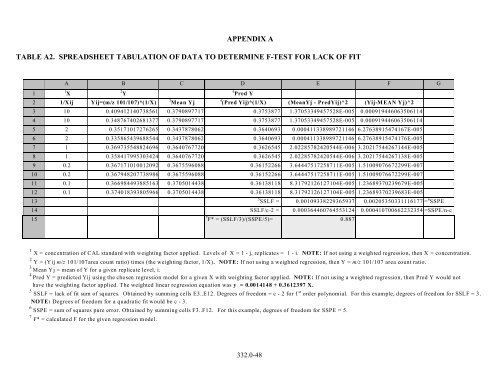
APPENDIX A
TABLE A2. SPREADSHEET TABULATION OF DATA TO DETERMINE F-TEST FOR LACK OF FIT
1 1 X
A B C D E F G
2 1/Xij Yij=(m/z 101/107)*(1/X)
2 Y
4 Pred Y
3 Mean Yj
4 (Pred Yij)*(1/X) (MeanYj - PredYij)^2 (Yij-MEAN Yj)^2
3 10 0.409412140738561 0.3790897717 0.3753877 1.37053349457528E-005 0.000919446063506114
4 10 0.348767402681377 0.3790897717 0.3753877 1.37053349457528E-005 0.000919446063506114
5 2 0.35171017276265 0.3437878062 0.3640693 0.000411338989721146 6.27638915474167E-005
6 2 0.335865439688544 0.3437878062 0.3640693 0.000411338989721146 6.27638915474176E-005
7 1 0.369735548824696 0.3640767720 0.3626545 2.02285782420544E-006 3.20217544267144E-005
8 1 0.358417995303424 0.3640767720 0.3626545 2.02285782420544E-006 3.20217544267138E-005
9 0.2 0.367171010012092 0.3675596088 0.36152266 3.64447517258711E-005 1.51009076672299E-007
10 0.2 0.367948207738986 0.3675596088 0.36152266 3.64447517258711E-005 1.51009076672299E-007
11 0.1 0.366984493885163 0.3705014438 0.36138118 8.31792126127104E-005 1.23689370239679E-005
12 0.1 0.374018393805966 0.3705014438 0.36138118 8.31792126127104E-005 1.23689370239683E-005
13 5 SSLF = 0.00109338229365937 0.00205350331116177 = 6 SSPE
14 SSLF/c-2 = 0.000364460764553124 0.000410700662232354 =SSPE/n-c
15
7 F* = (SSLF/3)/(SSPE/5)= 0.887
1
X = concentration of CAL standard with weighting factor applied. Levels of X = 1 - j, replicates = 1 - i. NOTE: If not using a weighted regression, then X = concentration.
2
Y = (Yij m/z 101/107area count ratio) times (the weighting factor, 1/X). NOTE: If not using a weighted regression, then Y = m/z 101/107 area count ratio.
3 Mean Yj = mean of Y for a given replicate level, i.
4 Pred Y = predicted Yij using the chosen regression model for a given X with weighting factor applied. NOTE: If not using a weighted regression, then Pred Y would not
have the weighting factor applied. The weighted linear regression equation was y = 0.0014148 + 0.3612397 X.
5 SSLF = lack of fit sum of squares. Obtained by summing cells E3..E12. Degrees of freedom = c - 2 for 1 st order polynomial. For this example, degrees of freedom for SSLF = 3.
NOTE: Degrees of freedom for a quadratic fit would be c - 3.
6 SSPE = sum of squares pure error. Obtained by summing cells F3..F12. For this example, degrees of freedom for SSPE = 5.
7
F* = calculated F for the given regression model.
332.0-48