Testing Distributional Dependence in the Becker-DeGroot-Marschak ...

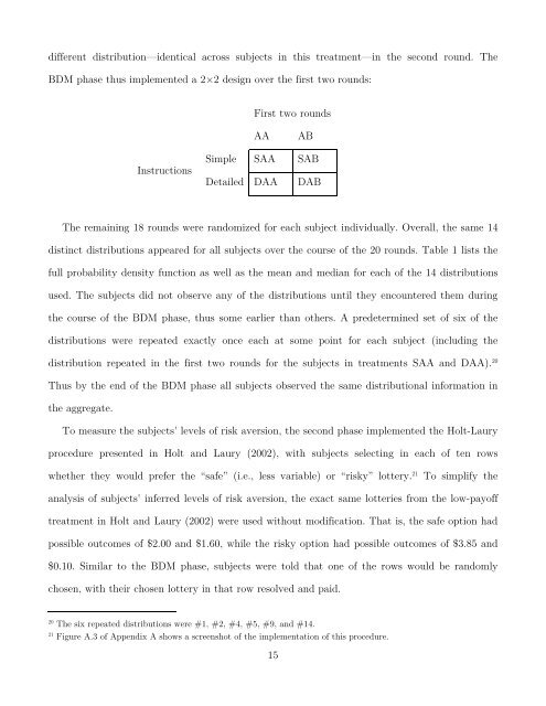
different distribution—identical across subjects in this treatment—in the second round. The
BDM phase thus implemented a 2×2 design over the first two rounds:
Instructions
First two rounds
AA AB
Simple SAA SAB
Detailed DAA DAB
The remaining 18 rounds were randomized for each subject individually. Overall, the same 14
distinct distributions appeared for all subjects over the course of the 20 rounds. Table 1 lists the
full probability density function as well as the mean and median for each of the 14 distributions
used. The subjects did not observe any of the distributions until they encountered them during
the course of the BDM phase, thus some earlier than others. A predetermined set of six of the
distributions were repeated exactly once each at some point for each subject (including the
distribution repeated in the first two rounds for the subjects in treatments SAA and DAA). 20
Thus by the end of the BDM phase all subjects observed the same distributional information in
the aggregate.
To measure the subjects' levels of risk aversion, the second phase implemented the Holt-Laury
procedure presented in Holt and Laury (2002), with subjects selecting in each of ten rows
whether they would prefer the “safe” (i.e., less variable) or “risky” lottery. 21 To simplify the
analysis of subjects' inferred levels of risk aversion, the exact same lotteries from the low-payoff
treatment in Holt and Laury (2002) were used without modification. That is, the safe option had
possible outcomes of $2.00 and $1.60, while the risky option had possible outcomes of $3.85 and
$0.10. Similar to the BDM phase, subjects were told that one of the rows would be randomly
chosen, with their chosen lottery in that row resolved and paid.
20 The six repeated distributions were #1, #2, #4, #5, #9, and #14.
21 Figure A.3 of Appendix A shows a screenshot of the implementation of this procedure.
15