the numerical sea ice forecast in finland in the winter 1993-94 ...

Sinte 1918 the Finnish Institute of Marine Research has provided a Baltic Sea sea ice information
service, shorted to Ice Service, in order to provide information on ice conditions and with the
cooperation of the Finnish Marine Administration, to coordinate winter navigation and make ice
breaking assistance as effective as possible (Grönvall 1988).
The Finnish Ice Service consists of three operative systems: ice observation network, ice analysis and
forecast system, and ice information communication system. Empirital-statistical schemes have been
traditionally used for operational ice forecasting based on the analysis of meteorologital and
oceanographic data and ice conditions.
In Finland the sea ice observation network was set up in the 1800’s. After the introduction of the first
icebreaker in 1890, need for knowledge of the almost unstudied sea ice rose fast. Field experiments,
however, were minimal until 1950’s when the sea ice field studies started at large. The practical need
for forecasting ice conditions sinte harbours of the Bothnian Bay have been kept open year around,
with the development of computer technology and sea ice physics in early 197O’s, has led to the
development of a numerical ice model. The model was in test use for first time in 1977, and in routine
use sinte 1978 (Leppäranta 1981). The model was tested widely and new information was collected
during annual field experiments and the first generation model was completed in 1984.
A joint Finnish-Chinese sea ice research project was founded in 1988 and a numerical sea ice model
for the Bohai Sea was developed (Wu & Leppäranta 1990; Wu et al. 1993). The model has been the
basis for developing a new Baltic Sea ice model.
Tests of the new model for forecasting ice conditions has been successfully carried out in Finland
during the winter 1993-94: the model was in operational use for 85 days in the Finnish Ice Service.
2. NUMERICAL ICE MODEL
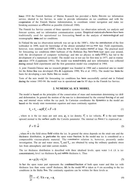
The model is based on the principles of the conservation of mass and momentum determining ice drift
and deformation. In general the motion of the sea ice is determinated by the external forting of air and
sea, and internal stress within the ice pack. In Cartesian coordinates the dynamits in the model are
based on the steady state momentum equation and mass continuity equation:
> where m is the ice mass per unit area, pi is ice density, < is ice velocity, K is the unit vector
upward normal to the surface andfis the Coriolis parameter. The internal ice forte F is expressed as
(1)
(2)
where å is the field stress field within the ice. In general the stress depends on the strait rate and the
ihickness distribution, in particular the open water fraction. In the model sea ice is considered as a
compressible viscous-plastic material. The constitutive relation is, however, presently under
investigation. The air and water stress, i, and ,, are obtained by using the ordinary quadratic stress
law from atmospheric and tidal current models.
The ice thickness distribution is described with three idealised levels: open water 1-A (A is ice
toncentration), leve1 ice thickness hl and rubble thickness h,. Thus
m=p;(4 +h)A (3)
In fatt the open water part represents the combined fraction of both open water and thin ice with
thickness less than some cutoff thickness, ho. In the model h0 is taken as 4 cm according to the ice
conditions in the Baltic Sea. The continuity equations can be written for three levels as
i3A
-=-q.vA+y~~+$,
at
(4)