here - UMSL : Mathematics and Computer Science - University of ...

IEEE TRANS. SIGNAL PROC. 1 

Orthogonal and Biorthogonal √ 3-refinement 

Wavelets for Hexagonal Data Processing 

Qingtang Jiang 

Abstract 

The hexagonal lattice was proposed as an alternative method for image sampling. The hexagonal sampling has 

certain advantages over the conventionally used square sampling. Hence, the hexagonal lattice has been used in 

many areas. 

A hexagonal lattice allows √ 3, dyadic and √ 7 refinements, which makes it possible to use the multiresolution 

(multiscale) analysis method to process hexagonally sampled data. The √ 3-refinement is the most appealing refinement 

for multiresolution data processing due to the fact that it has the slowest progression through scale, and hence, 

it provides more resolution levels from which one can choose. This fact is the main motivation for the study of 

√ 

3-refinement surface subdivision, and it is also the main reason for the recommendation to use the 

√ 

3-refinement 

for discrete global grid systems. However, there is little work on compactly supported √ 3-refinement wavelets. In 

this paper we study the construction of compactly supported orthogonal and biorthogonal √ 3-refinement wavelets. 

In particular, we present a block structure of orthogonal FIR filter banks with 2-fold symmetry and construct 

the associated orthogonal √ 3-refinement wavelets. We study the 6-fold axial symmetry of perfect reconstruction 

(biorthogonal) FIR filter banks. In addition, we obtain a block structure of 6-fold symmetric √ 3-refinement filter 

banks and construct the associated biorthogonal wavelets. 

Index Terms 

Hexagonal lattice, hexagonal image, filter bank with 6-fold symmetry, √ 3-refinement hexagonal filter bank, 

orthogonal √ 3-refinement wavelet, biorthogonal √ 3-refinement wavelet, √ 3-refinement multiresolution decomposition/reconstruction. 

EDICS Category: MRP-FBNK 

I. INTRODUCTION 

Images are conventionally sampled at the nodes on a square or rectangular lattice (array), and hence, traditional 

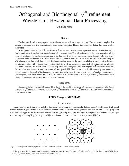
image processing is carried out on a square lattice. The hexagonal lattice (see the left part of Fig. 1) was proposed 

four decades ago as an alternative method for image sampling. The hexagonal sampling has certain advantages 

over the square sampling (see e.g. [1]-[8]), and hence, it has been used in many areas [9]-[20]. 

b 

Fig. 1. 

Hexagonal lattice (left) and its associated hexagonal tessellation (right) 

Q. Jiang is with the Department of Mathematics and Computer Science, University of Missouri–St. Louis, St. Louis, MO 63121, USA, 

e-mail: jiangq@umsl.edu , web: http://www.cs.umsl.edu/∼jiang .


For images/data sampled on a hexagonal lattice, each node on the hexagonal lattice represents a hexagonal cell 

with that node as its center. A node b and the hexagonal cell (called the elementary hexagonal cell) it represents 

are shown in the right part of Fig. 1. All the hexagonal elementary cells form a hexagonal tessellation of the plane. 

It was shown in [21], [22] that a hexagonal lattice allows three interesting types of refinements: 3-size (3-branch, 

or 3-aperture), 4-size (4-branch, or 4-aperture) and 7-size (7-branch, or 7-aperture) refinements. In the left picture 

of Fig. 2, the nodes of the unit regular hexagonal lattice G are denoted by black dots • and the nodes with circles ○ 

form a new lattice, which is called the 4-size (4-branch, or 4-aperture) sublattice of G here and it is denoted by G 4 . 

G 4 is also a regular hexagonal lattice. From G to G 4 , the nodes are reduced by a factor 1 4 . So G 4 is a coarse lattice 

of G, and G is a refinement of G 4 . Since G 4 is also a regular hexagonal lattice, we can repeat the same procedure 

to G 4 , and we then have a high-order (coarse) regular hexagonal lattice with fewer nodes than G 4 . Repeating this 

procedure, we have a set of lattices with fewer and fewer nodes. This set of lattices forms a “pyramid” or “tree” 

with a high-order lattice has fewer nodes than its predecessor by a factor of 1 4 

. The hexagonal tessellation associated 

with G 4 (nodes of G 4 are the centroids of hexagons (with thick edges) to form the tessellation) is shown in the right 

picture of Fig. 2, where the hexagonal tessellation associated with G (with thin hexagon edges) is also provided. 

Fig. 2. Left picture: Hexagonal lattice G (consisting of nodes •) and its 4-size sublattice G 4 (consisting of nodes ○); Right 

picture: hexagonal tessellations associated with G and G 4 

Fig. 3. Left picture: Hexagonal lattice G (consisting of nodes •) and its 3-size sublattice G 3 (consisting of nodes ○); Right 

picture: Hexagonal tessellations associated with G and G 3 

In the left picture of Fig. 3, the nodes with circles ○ form a new coarse lattice, which is called the 3-size 

(3-branch, or 3-aperture) sublattice of G here, and it is denoted by G 3 . From G to G 3 , the nodes are reduced by a 

factor 1 3 

. Again, repeating this process, we have a set of regular lattices which forms a “pyramid”. The hexagonal 

tessellation associated with G 3 is shown in the right picture of Fig. 3. The reader refers to [23] for the 7-size 

refinement. 

Notice that the distances between any two (nearest) adjoint nodes in G 3 and G 4 are respectively √ 3 and 2. 

The 3-size and 4-size refinements are called respectively √ 3 and dyadic (or 1-to-4 split) refinements in the area 

of Computer Aided Geometry Design [24]-[30], while they are called aperture 3 and aperture 4 (refinements) in 

discrete global grid systems in [20].


The refinements of the hexagonal lattice allow the multiresolution (multiscale) analysis method to be used to 

process hexagonally sampled data. The dyadic (4-size) refinement is the most commonly used refinement for 

multiresolution image processing, and there are many papers on the construction and/or applications of dyadic 

hexagonal filter banks and wavelets, see e.g. [11], [12], [18], [31]-[37]. Though √ 7-refinement (7-size refinement) 

has some special properties, the √ 7-refinement multiresolution data processing results in a reduction in resolution 

by a factor 7 which may be too coarse and is undesirable. The reader refers to [23] for the construction of √ 7- 

refinement wavelets. 

The √ 3 (3-size) refinement is the most appealing refinement for multiresolution data processing due to the fact 

that √ 3-refinement generates more resolutions and, hence, it gives applications more resolutions from which to 

choose. This fact is the main motivation for the study of √ 3-refinement subdivision in [24]-[30] and it is also 

the main reason for the recommendation to use the √ 3-refinement for discrete global grid systems in [20], where 

√ 

3-refinement is called 3 aperture. The 

√ 

3-refinement has been used by engineers and scientists of the PYXIS 

innovation Inc. to develop The PYXIS Digital Earth Reference Model [38]. However, there is little work on √ 3- 

refinement wavelets. [40], [41] are the only articles available in the literature on this topic. (The readers to [39] for 

rotation covariant quincunx wavelets on square lattice.) The authors of [41] construct biorthogonal √ 3-refinement 

wavelets by adopting the method in [35] for the construction of dyadic wavelets. The wavelets in [35] and [41] 

are constructed for the purpose of surface multiresolution processing which involves both regular and extraordinary 

nodes (vertices) in the surfaces. It is hard to calculate the L 2 inner product of the scaling functions (also called 

basis functions) and wavelets associated with extraordinary nodes. Thus, when considering the biorthogonality, [35] 

and [41] do not use the L 2 inner product. Instead, they use a “discrete inner product” related to the discrete filters. 

That discrete inner product may result in basis functions and wavelets which are not L 2 (IR 2 ) functions. Indeed, the 

√ 

3-refinement analysis basis functions and wavelets (even associated with regular nodes) constructed in [41] are 

not in L 2 (IR 2 ), and hence they cannot generate Riesz bases for L 2 (IR 2 ). In this paper we study the construction of 

orthogonal and biorthogonal √ 3-refinement wavelets (for regular nodes) with the conventional L 2 inner product. 

The rest of this paper is organized as follows. In Section II, we provide √ 3-refinement multiresolution decomposition 

and reconstruction algorithms and some basic results on the orthogonality/biorthogonality of √ 3-refinement 

filter banks. In Section III, we study the construction of orthogonal √ 3-refinement wavelets. We will present a 

block structure of orthogonal FIR filter banks. In Section IV, we address the construction of √ 3-refinement perfect 

reconstruction (biorthogonal) filter banks with 6-fold axial symmetry and the associated biorthogonal wavelets. 

In this paper we use bold-faced letters such as k, x, ω to denote elements of Z 2 and IR 2 . A multi-index k of Z 2 

and a point x in IR 2 will be written as row vectors 

k = (k 1 , k 2 ), x = (x 1 , x 2 ). 

However, k and x should be understood as column vectors [k 1 , k 2 ] T and [x 1 , x 2 ] T when we consider Ak and Ax, 

where A is a 2×2 matrix. For a matrix M, we use M ∗ to denote its conjugate transpose M T , and for a nonsingular 

matrix M, M −T denotes (M −1 ) T . 

II. MULTIRESOLUTION PROCESSING WITH 

√ 

3-REFINEMENT FILTER BANKS 

In this section, we provide √ 3-refinement multiresolution decomposition and reconstruction algorithms and 

present some basic results on the orthogonality/biorthogonality of √ 3-refinement filter banks. 

A. √ 3-refinement multiresolution algorithms 

Let G denote the regular unit hexagonal lattice defined by 

where 

G = {k 1 v 1 + k 2 v 2 : k 1 , k 2 ∈ Z}, (1) 

v 1 = [1, 0] T , v 2 = [− 1 2 , √ 

3 

2 ]T . 

To a node g = k 1 v 1 +k 2 v 2 of G, we use (k 1 , k 2 ) to indicate g, see the left part of Fig. 4 for the labelling of G. Thus, 

for hexagonal data c sampled on G, instead of using c g , we use c k1 ,k 2 

to denote the pixel of c at g = k 1 v 1 + k 2 v 2 .


02 12 

22 

−11 01 11 21 

v 2 

00 

−20 −10 v 1 10 20 

−2−1 −1−1 0−1 1−1 

−2−2 

−1−2 

0−2 

c 

−20 

c 

12 

22 

c −11 01 c11 

c21 

c 

c −2−1 

c 02 

c 

−10 

c 

−2−2 

−1−1 

c 

c 

c 

00 

c 

−1−2 

0−1 

c 

c 

c 

10 

0−2 

c 

c 1−1 

20 

Fig. 4. 

Left: Indices for hexagonal nodes; Right: Indices for hexagonally sampled data c 

Therefore, we write c, data hexagonally sampled on G, as c = {c k1,k 2 

} k1,k 2∈Z, see the right part of Fig. 4 for c k1,k 2 

. 

Denote 

Then the coarse lattice G 3 is generated by 

V 1 = 2v 1 + v 2 , V 2 = −v 1 + v 2 . 

G 3 = {k 1 V 1 + k 2 V 2 : 

k 1 , k 2 ∈ Z}. 

Observe that k 1 V 1 + k 2 V 2 = (2k 1 − k 2 )v 1 + (k 1 + k 2 )v 2 . Thus, the indices for nodes of G 3 are {(2k 1 − k 2 , k 1 + 

k 2 ), k 1 , k 2 ∈ Z} and hence, the data c associated with G 3 is given by {c (2k1−k 2,k 1+k 2)} k1,k 2∈Z. 

To provide the multiresolution image decomposition and reconstruction algorithms, we need to choose a 2 × 2 

matrix M, called the dilation matrix, such that it maps the indices for the nodes of the hexagonal lattice G onto 

those for the nodes of the coarse lattice G 3 , namely, we need to choose M such that 

M : (k 1 , k 2 ) → (2k 1 − k 2 , k 1 + k 2 ), k 1 , k 2 ∈ Z. 

One may choose M to be a matrix that maps A = {(1, 0), (1, 1), (0, 1), (−1, 0), (−1, −1), (0, −1)} onto B = 

{(2, 1), (1, 2), (−1, 1), (−2, −1), (−1, −2), (1, −1)}. Notice that k 1 v 1 + k 2 v 2 with (k 1 , k 2 ) ∈ A form a hexagon, 

while k 1 v 1 + k 2 v 2 with (k 1 , k 2 ) ∈ B form a hexagon with vertices in G 3 . There are several choices for such a 

matrix M. Here we consider two of such matrices (refer to [29] for other choices of M): 

[ ] [ ] 

2 −1 

2 −1 

M 1 = 

, M 

1 1 

2 = 

(2) 

1 −2 

As sets, both M 1 Z 2 and M 2 Z 2 are the same set {(2k 1 − k 2 , k 1 + k 2 ) : k 1 , k 2 ∈ Z}: the indices for nodes 

in the coarse lattice G 3 . But considering the individual nodes of G 3 with indices M 1 k, k ∈ Z 2 and those with 

M 2 k, k ∈ Z 2 , one observes that the coarse lattice of nodes with M 1 k, k ∈ Z 2 keeps the orientation but is rotated 

clockwise 30 ◦ with respect to the axes of G (see the left part of Fig. 5, where a 1 , · · · , f 1 are the images of a, · · · , f 

with M 1 ), while the coarse lattice of nodes with M 2 k, k ∈ Z 2 are rotated and reflected from those of G (see the 

right part of Fig. 5, where a 2 , · · · , f 2 are the images of a, · · · , f with M 2 ). One also observes that the axes of the 

coarser lattice of nodes with M2 2k, k ∈ Z2 are the same as those of G since (M 2 ) 2 = 3I 2 . In [42], the subsampling 

such as that with M 1 (M 2 respectively) is called the spiraling (toggling respectively) subsampling. It should be up 

to one’s specific application to use M 1 , M 2 or another dilation matrix. 

For a sequence {p k } k∈Z 

2 of real numbers with finitely many p k nonzero, let p(ω) denote the finite impulse 

response (FIR) filter with its impulse response coefficients p k (here a factor 1/3 is added for convenience): 

p(ω) = 1 ∑ 

p k e −ik·ω . 

3 

k∈Z 2 

When k, k ∈ Z 2 , are considered as indices for nodes g = k 1 v 1 + k 2 v 2 of G, p(ω) is a hexagonal filter, see Fig. 6 

for the coefficients p k1,k 2 

. In this paper, a filter means a hexagonal filter though the indices of its coefficients are 

given by k with k in the square lattice Z 2 .


b1 

f 

2 

c 1 

d 1 

d 

c 

e 

b 

a 1 

a 

f f 1 

e 1 

e 

d 2 

2 

d 

c 

e 

c 

b 

f 

2 

a 

a 

b 

2 

2 

Fig. 5. 

Hexagonal lattice with √ 3 spiraling refinement (left) and hexagonal lattice with √ 3 toggling refinement (right) 

p −20 

p−2−1 

p 

02 

p p 22 

p −11 p 01 

p 11 p 

21 

p −10 

p 00 

p 10 

p 

20 

p −2−2 

p −1−1 

12 

p −1−2 

p 

0−1 

p 

0−2 

p 

1−1 

Fig. 6. Indices for impulse response coefficients p k1,k 2 

For a pair of filter banks {p(ω), q (1) (ω), q (2) (ω)} and {˜p(ω), ˜q (1) (ω), ˜q (2) (ω)}, the multiresolution decomposition 

algorithm with a dilation matrix M for an input hexagonally sampled image c 0 k 

{ 

is 

c j+1 

n = (1/3) ∑ k∈Z p k−Mnc j 2 k , 

d (l,j+1) 

n 

= (1/3) ∑ k∈Z 2 q(l) k−Mn cj k , (3) 

with l = 1, 2, n ∈ Z 2 for j = 0, 1, · · · , J − 1, and the multiresolution reconstruction algorithm is given by 

ĉ j k = ∑ ˜p k−Mn ĉ j+1 

n + ∑ ∑ 

n (4) 

n∈Z 2 

1≤l≤2 

n∈Z 2 ˜q (l) 

k−Mn d(l,j+1) 

with k ∈ Z 2 for j = J − 1, J − 2, · · · , 0, where ĉ n,J = c n,J . We say hexagonally filter banks {p, q (1) , q (2) } and 

{˜p, ˜q (1) , ˜q (2) } to be the perfect reconstruction (PR) filter banks if ĉ j k = cj k 

, 0 ≤ j ≤ J − 1 for any input hexagonally 

sampled image c 0 k . {p, q(1) , q (2) } is called the analysis filter bank and {˜p, ˜q (1) , ˜q (2) } the synthesis filter bank. 

From (3) and (4), we know when the indices of hexagonally sampled data are labelled by (k 1 , k 2 ) ∈ Z 2 as 

in Fig. 4, the decomposition and reconstruction algorithms for hexagonal data with hexagonal filter banks are the 

conventional multiresolution decomposition and reconstruction algorithms for squarely sampled images. Thus, the 

integer-shift invariant multiresolution analysis theory implies (refer to e.g. [43]) that {p, q (1) , q (2) } and {˜p, ˜q (1) , ˜q (2) } 

are PR filter banks if and only if 

∑ 

p(ω + 2πM −T η k )˜p(ω + 2πM −T η k ) = 1, (5) 

0≤k≤2 

∑ 

0≤k≤2 

∑ 

0≤k≤2 

p(ω + 2πM −T η k )˜q (l) (ω + 2πM −T η k ) = 0, (6) 

q (l′) (ω + 2πM −T η k )˜q (l) (ω + 2πM −T η k ) = δ l′ −l, (7)


for 1 ≤ l, l ′ ≤ 2, ω ∈ IR 2 , where η j , 0 ≤ j ≤ 2 are the representatives of the group Z 2 /(M T Z 2 ), δ k is the 

kronecker-delta sequence: δ k = 1 if k = 0, and δ k = 0 if k ≠ 0. When M is the dilation matrix M 1 or M 2 in (2), 

we may choose η j , 0 ≤ j ≤ 2 to be 

η 0 = (0, 0), η 1 = (1, 0), η 2 = (−1, 0). (8) 

Filter banks {p, q (1) , q (2) } and {˜p, ˜q (1) , ˜q (2) } are also said to be biorthogonal if they satisfy (5)-(7); and a filter 

bank {p, q (1) , q (2) } is said to be orthogonal if it satisfies (5)-(7) with ˜p = p, ˜q (l) = q (l) , 1 ≤ l ≤ 2. 

Let {p, q (1) , q (2) } and {˜p, ˜q (1) , ˜q (2) } be a pair of FIR filter banks. Let φ and ˜φ be the scaling functions (with 

dilation matrix M) associated with lowpass filters p(ω) and ˜p(ω) respectively, namely, φ, ˜φ satisfy the refinement 

equations: 

φ(x) = ∑ k∈Z 2 p k φ(Mx − k), ˜φ(x) = ∑ k∈Z 2 ˜p k ˜φ(Mx − k), (9) 

and ψ (l) , ˜ψ (l) , 1 ≤ l ≤ 2 are given by 

ψ (l) (x) = ∑ k∈Z 2 q(l) k 

φ(Mx − k), 

˜ψ (l) (x) = ∑ k∈Z 2 ˜q(l) ˜φ(Mx k 

− k), 

where p k , ˜p k , q (l) 

k , ˜q(l) k 

are the impulse response coefficients of p(ω), ˜p(ω), q(l) (ω), ˜q (l) (ω), respectively 

If {p, q (1) , q (2) } and {˜p, ˜q (1) , ˜q (2) } are biorthogonal to each other (with dilation M), then under certain mild 

conditions (see e.g. [44], [45], [43], [23]), φ and ˜φ are biorthogonal duals: ∫ IR φ(x)˜φ(x − k) dx 

2 

= δ k , k ∈ Z 2 , where δ k = δ k1 δ k2 . In this case, ψ (l) , ˜ψ (l) , l = 1, 2, are biorthogonal wavelets, namely, {ψ (l) 

j,k : l = 

1, 2, j ∈ Z, k ∈ Z 2 (l) 

} and { ˜ψ 

j,k : l = 1, 2, j ∈ Z, k ∈ Z2 } are Riesz bases of L 2 (IR 2 ) and they are biorthogonal to 

each other: 

∫ 

ψ (l) 

j,k (x) ˜ψ (l′ ) 

j ′ ,k 

(x)dx = δ ′ j−j ′δ l−l ′δ k−k ′, 

IR 2 

for j, j ′ ∈ Z, 1 ≤ l, l ′ ≤ 2, k, k ′ ∈ Z 2 , where 

ψ (l) 

j,k (x) = 3 j 2 ψ (l) (M j x − k), ˜ψ(l) j,k (x) = 3 j 2 ˜ψ(l) (M j x − k), j ∈ Z, k ∈ Z 2 . 

Remark 1: One can verify that {M1 −T η j : j = 0, 1, 2} = {M2 −T η j : j = 0, 1, 2}, where η j , j = 0, 1, 2 are 

the representatives for both Z 2 /M1 T Z2 and Z 2 /M2 T Z2 given in (8). Thus, {p, q (1) , q (2) } and {˜p, ˜q (1) , ˜q (2) } are 

biorthogonal with one of M 1 , M 2 , say M 1 , then they are also biorthogonal to each other with the other dilation 

matrix, M 2 . 

φ and ˜φ are refinable functions along Z 2 . φ, ˜φ and ψ (l) , ˜ψ (l) , l = 1, 2 are the conventional scaling functions and 

wavelets. Let U be the matrix defined by [ √ ] 

1 3 

Then U transforms the regular unit hexagonal lattice G onto the square lattice Z 2 . Define 

U = 

0 

3 

2 √ 3 

3 

Φ(x) = φ(Ux), Ψ (l) (x) = ψ (l) (Ux), 

˜Φ(x) = ˜φ(Ux), ˜Ψ (l) (x) = ˜ψ (l) (Ux), l = 1, 2. 

Then Φ and ˜Φ are refinable along G with the same coefficients p k and ˜p k for φ and ˜φ, and Ψ (l) , l = 1, 2 and 

˜Ψ (l) , l = 1, 2 are hexagonal biorthogonal wavelets (along the hexagonal lattice G). The reader refers to [46] for 

refinable functions along a general lattice. 

In the rest of this section, we give the definitions of the symmetries of filter banks considered in this paper. 

Definition 1: A hexagonal filter bank {p, q (1) , q (2) } is said to have 2-fold rotational symmetry if its lowpass filter 

p(ω) is invariant under π rotation, and its second highpass filter q (2) is the π rotation of its first highpass filter q (1) . 

Definition 2: Let S j , 0 ≤ j ≤ 5 be the axes in the left part of Fig. 7. A hexagonal filter bank {p, q (1) , q (2) } 

is said to have 6-fold axial symmetry or 6-fold line symmetry if (i) its lowpass filter p(ω) is symmetric around 

. 

(10) 

(11)


S 0 

S 0" 

S 1 

v 2 

v 1 S2 

S 3 

S 4 

11 

00 10 

20 

S2 

0−1 

S 5 

" 

S4 

Fig. 7. Left: 6 axes (lines) of symmetry for lowpass filter p; Right: 3 axes (lines) of symmetry for highpass filter q (1) 

S 0 , · · · , S 5 , (ii) its highpass filter satisfies that e −iω 1 q(1) (ω) is symmetric around the axes S 0 , S 2 , S 4 , and (iii) the 

other highpass filter q (2) is the π rotation of highpass filter q (1) . 

The right part of Fig. 7 shows the symmetry of q (1) , namely, q (1) is symmetric around the axes S 0 ′′, 

S 2, S 4 ′′, 


S 0 ′′ 

and S′′ 4 are the 1-unit right shifts of S 0 and S 4 respectively. 

The symmetry of hexagonal filter banks is important for image/data processing, and it leads to simpler algorithms 

and efficient computations. Unlike the orthogonal dyadic refinement and √ 7-refinement hexagonal filter banks which 

may have 3-fold and 6-fold symmetry respectively, it seems hard to construct orthogonal √ 3-refinement filter banks 

with high symmetry (only 2-fold symmetry can be obtained here). While for biorthogonal filter banks, we have 

more flexibility for their construction and very high symmetry can be gained. Some 3-direction box-splines in 

[47] are symmetric around S j , 0 ≤ j ≤ 5, and such box-splines are called to have the full set of symmetries. 

For the biorthogonal filter banks considered in this paper, the lowpass filters have the full set of symmetries, and 

the highpass filters also have certain symmetry as well. Such a symmetry of our filter banks not only results in 

efficient computations, but also makes it possible to design surface multiresolution decomposition and reconstruction 

algorithms for extraordinary nodes when the filters constructed in this paper are used for the multiresolution 

algorithms for regular nodes. More precisely, our symmetric biorthogonal filter banks result in multiresolution 

algorithms independent of the orientation of the nodes. This is critical for the design of multiresolution algorithms for 

extraordinary nodes in multiresolution surface processing. The design of multiresolution algorithms for extraordinary 

nodes will appear elsewhere. 

In the next section, Section III, we discuss the construction of 2-fold symmetric orthogonal √ 3-refinement 

wavelets, and in Section IV, we consider the construction of 6-fold symmetric biorthogonal √ 3-refinement wavelets. 

When we consider orthogonal and biorthogonal wavelets, from Remark 1, we need only to consider one of the 

dilation matrices M 1 , M 2 . In the rest of this paper, without loss of generality, we choose M to be M 1 . 

III. ORTHOGONAL 

√ 

3-REFINEMENT WAVELETS 

In this section we consider filter banks with 2-fold rotational symmetry. First we give a family of 2-fold symmetric 

orthogonal filter banks. 

By the definition of the symmetry, we know that an FIR filter bank {p, q (1) , q (2) } has 2-fold rotational symmetry 

if and only if 

namely, 

or equivalently, 

p −k = p k , q (2) 

k 

= q(1) −k , k ∈ Z2 , 

p(−ω) = p(ω), q (2) (ω) = q (1) (−ω), ω ∈ IR 2 , 

[ 

p, q (1) , q (2)] T 

(−ω) = M0 

[ 

p(ω), q (1) (ω), q (2) (ω) ] T 

, (12) 


⎡ 

M 0 = ⎣ 

1 0 0 

0 0 1 

0 1 0 

⎤ 

⎦ . (13)


We hope to construct filter banks {p, q (1) , q (2) } given by the product of appropriate block matrices. If we can write 

a symmetric FIR filter bank [p(ω), q (1) (ω), q (2) (ω)] T as a product B(M T ω)[p s (ω), q s (1) (ω), q s 

(2) (ω)] T , where M 

is M 1 defined in (2), B(ω) is a 3 × 3 matrix whose entries are trigonometric polynomials, and {p s , q s (1) , q s 

(2) } is 

another FIR filter bank with 2-fold rotational symmetry, then (12) implies that B(ω) satisfies 

where M 0 is the matrix defined by (13). 

Denote 

B(−M T ω) = M 0 B(M T ω)M −1 

0 , (14) 

I 0 (ω) = [1, e −iω1 , e iω1 ] T . (15) 

Clearly, I 0 (ω) satisfies (12). Therefore, 1-tap filter bank {1, e −iω 1 , eiω 1 

} has 2-fold rotational symmetry, and it 

could be used as the initial symmetric filter bank. 

Denote 

D 1 (ω) = diag(1, e −iω2 , e iω2 ), 

D 1 (ω) = diag(1, e −i(ω 1+ω ) 2 

, e i(ω 1+ω ) 2 

), 

(16) 

D 3 (ω) = diag(1, e −iω 1 , eiω 1 ). 

Then one can easily verify that D 1 (ω), D 2 (ω), D 3 (ω), D 1 (−ω), D 2 (−ω), D 3 (−ω) satisfy (14), and thus they 

could be used to build the block matrices. Next we use B(ω) = BD(ω) as the block matrix, where B is a 3 × 3 

(real) constant matrix, and D(ω) is D j (ω) or D j (−ω) for some j, 1 ≤ j ≤ 3. Based on the above discussion, we 

know that B(ω) = BD(ω) satisfies (14) if and only if B satisfies M 0 BM0 −1 = B, which is equivalent to that B 

has the form: 

⎡ 

⎤ 

b 11 b 12 b 12 

B = ⎣ b 21 b 22 b 23 

⎦ . (17) 

b 21 b 23 b 22 

Thus we conclude that if {p, q (1) , q (2) } is given by 

[p(ω), q (1) (ω), q (2) (ω)] T = 1 √ 

3 

B n D(M T ω)B n−1 D(M T ω) · · · B 1 D(M T ω)B 0 I 0 (ω) (18) 

for some n ∈ Z + , where I 0 (ω) is defined by (15), B k , 0 ≤ k ≤ n are constant matrices of the form (17), and each 

D(ω) is D j (ω) or D j (−ω) for some j, 1 ≤ j ≤ 3, then {p, q (1) , q (2) } is an FIR filter bank with 2-fold rotational 

symmetry. 

Next, we show that the block structure in (18) yields 2-fold symmetric orthogonal FIR filter banks. 

For an FIR filter bank {p, q (1) , q (2) }, denote q (0) (ω) = p(ω). Let U(ω) be a 3 × 3 matrix defined by U(ω) = 

[ 

q (l) (ω + η j ) ] 0≤l,j≤2 ,where η 0, η 1 , η 2 are given in (8). Then {p, q (1) , q (2) } is orthogonal if U(ω) is unitary for 

all ω ∈ IR 2 , that is it satisfies 

U(ω)U(ω) ∗ = I 3 , ω ∈ IR 2 . (19) 

Next, we write q (l) (ω), 0 ≤ l ≤ 2 as 

q (l) (ω) = √ 1 ( 

) 

q (l) 

0 (M T ω) + q (l) 

1 (M T ω)e −iω 1 

+ q (l) 

2 (M T ω)e iω 1 

, 

3 

where q (l) 

k 

(ω) are trigonometric polynomials. Let V (ω) denote the polyphase matrix (with dilation matrix M) of 

{p(ω), q (1) (ω), q (2) (ω)}: 

⎡ 

p 0 (ω) p 1 (ω) p 2 (ω) 

⎢ 

V (ω) = ⎣ q (1) 

0 (ω) q(1) 1 (ω) q(1) 2 (ω) ⎥ 

⎦ . (20) 

From the facts that 

q (2) 

0 

(ω) q(2) 1 

(ω) q(2) 

2 (ω) ⎤ 

[p(ω), q (1) (ω), q (2) (ω)] T = 

1 √ 

3 

V (M T ω)I 0 (ω),


where I 0 (ω) is defined by (15), and that the 3 × 3 matrix 1 √ 

3 

[I 0 (ω + 2πM −T η 0 ), I 0 (ω + 2πM −T η 1 ), I 0 (ω + 

2πM −T η 2 )] is unitary for all ω ∈ IR 2 , we know that (19) holds if and only if V (ω) is unitary for all ω ∈ IR 2 , 

namely, V (ω) satisfies 

V (ω)V (ω) ∗ = I 3 , ω ∈ IR 2 . (21) 

If {p, q (1) , q (2) } is given by (18), then its polyphase matrix V (ω) is 

V (ω) = B n D(ω)B n−1 D(ω) · · · B 1 D(ω)B 0 . 

Since each D(ω) is unitary, we know that if constant matrices B k , 0 ≤ k ≤ n, are orthogonal, then V (ω) satisfies 

(21). 

Next, we consider the orthogonality of a matrix B of the from (17). To this regard, let U denote the unitary 

matrix: 

⎡ 

⎤ 

U = 

⎢ 

⎣ 

1 0 0 

0 

1 √2 

1 √2 

0 

1 √2 − 1 √ 

2 

Then 

⎡ √ ⎤ 

b 11 

UBU ∗ √ 2b12 0 

= ⎣ 2b21 b 22 + b 23 0 ⎦ . 

0 0 b 22 − b 23 

[ √ ] 

b 

Thus B is orthogonal if and only if 11 2b12 

√2b21 is orthogonal and b 22 + b 23 = ±1, which implies that 

b 22 + b 23 

b ij can be written as 

⎥ 

⎦ . 

b 11 = s 0 cos θ, b 12 = 1 √ 

2 

sin θ, b 21 = s 0 

√ 

2 

sin θ, 

b 22 + b 23 = − cos θ, b 22 − b 23 = s 1 , 

where s 0 = ±1, s 1 = ±1, θ ∈ IR. Thus an orthogonal matrix B of the form (17) has one parameter. If we choose 

s 0 = 1, s 1 = 1 and write cos θ = 1−t2 

1+t 

, sin θ = 2t 

2 1+t 

, then we have 

2 

√ 

b 11 = 1−t2 

1+t 

, b 2 12 = b 21 = 2t 

1+t 

, b 2 22 = t2 

1+t 

, b 2 23 = 1 

1+t 

. (23) 

2 

We have therefore the following theorem. 

Theorem 1: Suppose {p, q (1) , q (2) } is given by (18). If each B k , 0 ≤ k ≤ n is of the form (17) and its entries b ij 

are given by (22) for some θ k , then {p, q (1) , q (2) } is an orthogonal FIR filter bank with 2-fold rotational symmetry. 

With such a family of orthogonal FIR filter banks, by selecting the free parameters, one can design the filters 

with desirable properties. Here we consider the filters based on the Sobolev smoothness of the associated scaling 

functions φ. We say φ to be in the Sobolev space W s for some s > 0 if φ satisfies ∫ IR 2(1 + |ω|2 ) s | ˆφ(ω)| 2 dω < ∞. 

To assure that φ ∈ W s , the associated FIR lowpass filter p(ω) has sum rules of certain order. p(ω) is said to have 

sum rule order m (with dilation matrix M) provided that p(0, 0) = 1 and 

(22) 

D α 1 

1 Dα 2 

2 p(2πM −T η j ) = 0, 1 ≤ j ≤ 2, (24) 

for all (α 1 , α 2 ) ∈ Z 2 + with α 1 + α 2 < m, where η j , 1 ≤ j ≤ 2, are defined by (8), D 1 and D 2 denote the 

partial derivatives with the first and second variables of p(ω) respectively. Under some condition, sum rule order is 

equivalent to the approximation order of φ, see [48]. The Sobolev smoothness of φ can be given by the eigenvalues 

of the so-called transition operator matrix T p associated with the lowpass filter p, see [49], [50]. The reader refers 

to [26] for the algorithms and Matlab routines to find the Sobolev smoothness order. 

We find that if the orthogonal filter bank {p, q (1) , q (2) } is given by (18) with n = 0 or n = 1, then the lowpass 

filter p(ω) cannot achieve sum rule order 2, and hence, the smoothness order of φ is very low. In the following 

two examples, we consider the filter banks with n = 2 and n = 3. 

Example 1: Let {p, q (1) , q (2) } be the orthogonal filter bank with 2-fold rotational symmetry given by (18) for 

n = 2: B 2 D 2 (M T ω)B 1 D 1 (M T ω)B 0 I 0 (ω), where D 1 , D 2 are defined in (16), B 0 , B 1 and B 2 are orthogonal


matrices of the form (17) with their entries b ij given by (23) for parameters t 0 , t 1 and t 2 respectively. The lowpass 

filter p(ω) depends on these three parameters t 0 , t 1 and t 2 . By solving the equations for sum rule order 2, we get 

√ 

2 

t 0 = − 

2 (3 + √ √ 

2 

19), t 1 = 

6 (−5 + √ √ 

2 

19), t 2 = − 

2 (5 + 3√ 3). 

The resulting scaling function φ with M = M 1 is in W 0.79282 . In Appendix A, we provide the resulting coefficients 

p k , q (1) 

k 

, q(2) k . The pictures for φ and ψ(1) are shown in Fig. 8 

From Remark 1, this resulting filter bank is orthogonal with dilation matrix M 2 . Furthermore, one can verify that 

the resulting p(ω) also has sum rule order 2 with M 2 . We find that the associated scaling function (with dilation 

M 2 ) is in W 0.80115 . ♦ 

Fig. 8. 

φ (left) and −ψ (1) (right) 

Example 2: Let {p, q (1) , q (2) } be the orthogonal filter bank with 2-fold rotational symmetry given by (18) for 

n = 3: B 3 D 1 (M T ω)B 2 D 2 (M T ω)B 1 D 1 (M T ω)B 0 I 0 (ω), where D 1 , D 2 are defined in (16), B 0 , B 1 , B 2 and B 3 are 

orthogonal matrices of the form (17) with their entries b ij given by (23) for parameters t 0 , t 1 , t 2 and t 3 respectively. 

If we choose, 

t 0 = −3.96188283176253, t 1 = −0.09286132100086, 

t 2 = −5.26430640532092, t 3 = 0.04994199850331, 

then the resulting p(ω) has sum rule order 2 (with both dilation matrices M 1 and M 2 ). The corresponding scaling 

function φ with M = M 1 is in W 0.84094 , and that with M = M 2 is in W 1.06523 . ♦ 

The orthogonal FIR filter banks given by (18) with more blocks B k D(M T ω) will produce wavelets with small 

increments of smoothness order. Similar to orthogonal dyadic refinement and √ 7-refinement hexagonal wavelets, 

we find it is also hard to construct orthogonal √ 3-refinement wavelets with high smoothness order. In the next 

section, we consider biorthogonal FIR filter banks, which give us some flexility for the construction of PR filter 

banks. 

In the rest of this section, we apply the filter bank in Example 1 to a hexagonally sampled image in the left part 

of Fig. 9. This is a part of the hexagonal image re-sampled from a 512 × 512 squarely sampled image Lena by 

the bilinear interpolation in [6]. The decomposed images (when M = M 1 ) with the lowpass filter p and highpass 

filters q (1) , q (2) are shown in the right part of Fig. 9 and in Fig. 10 respectively. These images are indeed rotated 

30 ◦ with respect to the original image. 

IV. BIORTHOGONAL 

√ 

3-REFINEMENT WAVELETS WITH 6-FOLD SYMMETRY 

In this section we consider the construction of biorthogonal √ 3-refinement FIR filter banks with 6-fold symmetry 

and the associated wavelets. In §IV.A, we present a characterization of symmetric filter banks. In §IV.B, we provide 

a family of 6-fold symmetric biorthogonal √ 3-refinement FIR filter banks and discuss the construction of the 

associated wavelets.


Fig. 9. 

Left: Original (hexagonal) image; Right: Decomposed image with lowpass filter p 

Fig. 10. 

Decomposed images with highpass filters q (1) (left) and q (2) (right) 

A. 6-fold axial symmetry 

Let 

and denote 

[ ] [ ] [ 0 1 

1 0 

1 −1 

L 0 = , L 

1 0 1 = 

, L 

1 −1 2 = 

0 −1 

L 3 = −L 0 , L 4 = −L 1 , L 5 = −L 2 , 

R 1 = 

[ 0 1 

−1 1 

Then for a j, 0 ≤ j ≤ 5, {p k } is symmetric around the symmetry axis S j in Fig. 7 if and only if p Lj k = p k ; and 

{p R1 k} is the π 3 (anticlockwise) rotation of {p k}. 

Observe that 

L j = (R 1 ) j L 0 , 0 ≤ j ≤ 5. 

Thus, instead of considering all L j , 0 ≤ j ≤ 5, we need only consider L 0 , R 1 when we discuss the 6-fold axial 

symmetry of a filter bank. First we have the following proposition. 

Proposition 1: A filter bank {p, q (1) , q (2) } has 6-fold axial symmetry if and only if it satisfies 

] 

. 

] 

, 

(25) 

[p, q (1) , q (2) ] T (R1 −T ω) = N 1 (ω)[p, q (1) , q (2) ] T (ω), (26) 

[p, q (1) , q (2) ] T (L 0 ω) = N 2 (ω)[p, q (1) , q (2) ] T (ω), (27) 


⎡ 

N 1 (ω) = ⎣ 

1 0 0 

0 0 e −i(2ω 1+ω 2 ) 

0 e i(2ω 1+ω 2 ) 

0 

⎤ 

⎡ 

⎦ , N 2 (ω) = ⎣ 

1 0 0 

0 e i(ω 1−ω 2 ) 

0 0 e −i(ω 1−ω 2 ) 

⎤ 

⎦ . (28) 

Proof. For a filter bank {p, q (1) , q (2) }, let h (1) (ω) = e iω 1 q(1) (ω), h (2) (ω) = e −iω 1 q(2) (ω). Then with the fact 

L j = R j 1 L 0, 0 ≤ j ≤ 5, we know {p, q (1) , q (2) } has 6-fold axial symmetry if and only if 

p(R1 −T ω) = p(L 0 ω) = p(ω), (29) 

h (1) ((R1 −T ) 2 ω) = h (1) ((R1 −T ) 4 ω) = h (1) (L 0 ω) = h (1) (ω), (30) 

h (2) (−ω) = h (1) (ω). (31)


Observe that R 3 1 = −I 2. This fact and (30) and (31) lead to that 

h (1) (R1 −T ω) = h (1) (−(R1 −T ) 4 ω) = h (1) (−ω) = h (2) (ω), 

h (2) (R1 −T ω) = h (2) (−(R1 −T ) 4 ω) = h (1) ((R1 −T ) 4 ω) = h (1) (ω), 

h (2) (L 0 ω) = h (1) (−L 0 ω) = h (1) (−ω) = h (2) (ω). 

Conversely, one can check that h (1) (R1 −T ω) = h (2) (ω), h (2) (R1 −T ω) = h (1) (ω) and h (2) (L 0 ω) = h (2) (ω) imply 

(30) and (31). Therefore, {p, q (1) , q (2) } has 6-fold axial symmetry if and only if 

[p, h (1) , h (2) ] T (R1 −T ω) = [p, h (2) , h (1) ] T (ω), (32) 

[p, h (1) , h (2) ] T (L 0 ω) = [p, h (1) , h (2) ] T (ω). (33) 

With h (1) (ω) = e iω 1 q(1) (ω), h (2) (ω) = e −iω 1 q(2) (ω), one can easily show that (26) and (27) are equivalent to (32) 

and (33). Hence, {p, q (1) , q (2) } has 6-fold axial symmetry if and only if (26) and (27) hold, as desired. ♦ 

Let M = M 1 . For an FIR filter bank {p, q (1) , q (2) }, let V (ω) be its polyphase matrix (with M = M 1 ) defined 

by (20). Based on Proposition 1, we reach the following proposition which gives the characterization of the 6-fold 

axial symmetry of a filter bank in terms of the corresponding polyphase matrix. 

Proposition 2: An FIR filter bank {p, q (1) , q (2) } has 6-fold axial symmetry if and only if its polyphase matrix 

V (ω) (with dilation matrix M = M 1 ) satisfies 

V (R1 −T ω) = N 0 (ω)V (ω)N 0 (ω), (34) 

V (L 0 ω) = J 0 V (ω)J 0 , (35) 


Proof. 

⎡ 

N 0 (ω) = ⎣ 

By the definition of V (ω), we have 

1 0 0 

0 0 e −iω 1 

0 e iω 1 

0 

⎤ 

⎡ 

⎦ , J 0 = ⎣ 

1 0 0 

0 0 1 

0 1 0 

⎤ 

⎦ . (36) 

[p, q (1) , q (2) ](R −T 

1 ω) = 1 √ 

3 

V (M T R −T 

1 ω)I 0 (R −T 

1 ω) = 1 √ 

3 

V (M T R −T 

1 ω)N 1 (ω)I 0 (ω). 

Thus (26) is equivalent to 

or equivalently, 

1 

√ 

3 

V (M T R −T 

1 ω)N 1 (ω)I 0 (ω) = N 1 (ω) 1 √ 

3 

V (M T ω)I 0 (ω), 

V (M T R −T 

1 ω)N 1 (ω) = N 1 (ω)V (M T ω). 

The fact M T R −T 

1 = R −T 

1 M T (M = M 1 ) leads to that the above equality is 

or, 

which is (34) because of the fact N 1 (M −T ω) = N 0 (ω). 

Similarly as above, we have that (27) is equivalent to 

V (R −T 

1 M T ω)N 1 (ω) = N 1 (ω)V (M T ω), 

V (R −T 

1 ω) = N 1 (M −T ω)V (ω)N 1 (M −T ω), 

V (M T L 0 ω) = N 2 (ω)V (M T ω)N 2 (ω) −1 . 

From M T L 0 = R −T 

1 L 0 M T (when M = M 1 ), we know that the above equality is 

or, 

V (R −T 

1 L 0 M T ω) = N 2 (ω)V (M T ω)N 2 (ω) −1 , 

V (R −T 

1 L 0 ω) = N 2 (M −T ω)V (ω)N 2 (M −T ω) T ,


which in turn is equivalent to (under the assumption (34)) 

V (L 0 ω) = N 0 (L 0 ω)V (R −T 

1 L 0 ω)(L 0 ω) 

= N 0 (L 0 ω)N 2 (M −T ω)V (ω)N 2 (M −T ω) T N 0 (L 0 ω) −1 = J 0 V (ω)J 0 . 

Therefore, (26) and (27) are equivalent to (34) and (35). ♦ 

In the next subsection, based on the characterization in Proposition 2 for the 6-fold symmetry of filter banks, we 

provide a family of biorthogonal FIR filter banks with such a type of symmetry. 

B. Biorthogonal √ 3-refinement wavelets 

In this subsection we use the notations: 

x = e −iω 1 

, y = e −iω 2 

. 

Thus an FIR filter p(ω) can be written as a polynomial of x, y. Denote 

⎡ 

d + c(x + xy + y + 1 x + 1 

xy + 1 y ) a(1 + 1 x + y) a(1 + x + 1 y ) ⎤ 

W (ω) = ⎣ 

c 

2a (1 + x + 1 y ) 1 0 ⎦ , (37) 

c 

2a (1 + 1 x + y) 0 1 

where a, c, d are constants with a ≠ 0, d ≠ 3c. Next we use W (ω) to build a block structure of biorthogonal FIR 

filter banks with 6-fold symmetry. The motivation for the choice of W (ω) is based on the following observation. 

Let [p(ω), q (1) (ω), q (2) (ω)] T = 1 3 W (M T ω)I 0 (ω), where I 0 (ω) is defined by (15). Then the nonzero coefficients 

p k and q (1) 

k 

are shown in Fig. 11 with f = c 

2a . Clearly this filter bank {p, q(1) , q (2) } has 6-fold axial symmetry. 

(One may verify directly that its polyphase matrix W (ω) satisfies (34) and (35)). If a = 1 3 , d = 2 3 , c = 1 

18 

, then the 

corresponding {p k } is the subdivision mask constructed in [24]. 

c 

c 

a 

a 

a 

c 

d 

00 

a 

a 

a 

c 

c 

f 

00 

1 

f 

f 

c 

Fig. 11. Left: lowpass filter coefficients p k ; Right: highpass filter coefficients q (1) 

k 

with f = c 

2a 

Except for the property that W (ω) produces a 6-fold symmetry filter bank, W (ω) has another important property: 

the determinant of W (ω) is d − 3c, a nonzero constant. Thus, the inverse of W (ω) is a matrix whose entries are 

also polynomials of x, y. More precisely, ˜W (ω) = (W (ω) −1 ) ∗ is given by 

⎡ 

˜W (ω) = 1 

d−3c × 

1 − c 

2a 

⎢ 

(1 + 1 x + y) 

⎣ −a(1 + x + 1 y ) d − 3 2 c + c 2 (x + xy + y + 1 x + 1 

xy + 1 y ) 

−a(1 + 1 x + y) 

− c 

2a (1 + x + 1 y ) 

c 

2 (1 + x + 1 y )2 

c 

2 (1 + 1 x + y)2 d − 3 2 c + c 2 (x + xy + y + 1 x + 1 

xy + 1 y ) ⎤ 

⎥ 

⎦ . 

Hence, {p, q (1) , q (2) } has a biorthogonal FIR filter bank {˜p, ˜q (1) , ˜q (2) } defined by [˜p(ω), ˜q (1) (ω), ˜q (2) (ω)] T = 

˜W (M T ω)I 0 (ω). In addition, one can check directly (or from the fact W (ω) satisfies (34) and (35)) that ˜W (ω) 

satisfies (34) and (35). Thus, {˜p, ˜q (1) , ˜q (2) } also has 6-fold axial symmetry. More general, we have the following 

result. 

(38)


Theorem 2: Suppose FIR filter banks {p, q (1) , q (2) } and {˜p, ˜q (1) , ˜q (2) } are given by 

[p(ω), q (1) (ω), q (2) (ω)] T = U n (M T ω)U n−1 (M T ω) · · · U 0 (M T ω)I 0 (ω), (39) 

[˜p(ω), ˜q (1) (ω), ˜q (2) (ω)] T = 1 3Ũn(M T ω)Ũn−1(M T ω) · · · Ũ0(M T ω)I 0 (ω) 

for some n ∈ Z + , where I 0 (ω) is defined by (15), each U k (ω) is a W (ω) in (37) or a ˜W (ω) in (38) for 

some parameters a k , b k , d k , and Ũk(ω) = (U k (ω) −1 ) ∗ is the corresponding ˜W (ω) in (38) or W (ω) in (37), then 

{p, q (1) , q (2) } and {˜p, ˜q (1) , ˜q (2) } are biorthogonal FIR filter bank with 6-fold axial symmetry. 

Next we consider the construction of biorthogonal √ 3-refinement wavelets based on the symmetric biorthogonal 

FIR filter banks given in (39). When we construct biorthogonal wavelets, we will intently construct the synthesis 

scaling function ˜φ to have a higher smoothness order, and the analysis scaling function φ to have a higher approximation 

order (or equivalently the analysis lowpass filter p(ω) to have a higher sum rule order). Approximation property 

of φ is very important for applications, see e.g. [51], [52]. If φ has approximation order K, then the decomposition 

algorithm with lowpass filter p(ω) preserves (discrete) polynomials of order K, and the decomposition algorithm 

with highpass filters q (1) (ω), q (2) (ω) annihilates (discrete) polynomials of order K. Smoothness of ˜φ is in general 

more important than that for φ since certain smoothness of ˜φ is required to assure the reconstructed image to have 

nice visual quality. 

First, we consider the filter banks given by (39) with n = 0. Let [p(ω), q (1) (ω), q (2) (ω)] T = ˜W 0 (M T ω)I 0 (ω) and 

[˜p(ω), ˜q (1) (ω), ˜q (2) (ω)] T = 1 3 W 0(M T ω)I 0 (ω), where ˜W 0 (ω) and W 0 (ω) are given by (38) and (37) respectively 

for some parameters a 0 , c 0 , d 0 . By solving the equations of sum rule order 1 for ˜p(ω), we have 

a 0 = 1 3 , d 0 = 1 − 6c 0 . (40) 

The resulting ˜p(ω) actually has sum rule order 2 (the conditions in (24) for ˜p(ω) with (α 1 , α 2 ) = (1, 0) and 

(α 1 , α 2 ) = (0, 1) are automatically satisfied because of the symmetry of ˜p(ω)). If in addition, we choose c 0 = 1 18 , 

then ˜p(ω) has sum rule order 3. This ˜p(ω) is the subdivision mask in [24]. However, in this case the resulting 

p(ω) does not have sum rule order 1. With a 0 , d 0 given by (40) for some c 0 , by solving the equations of sum rule 

order 1 for p(ω), we have c 0 = − 2 9 . However, in this case the corresponding ˜φ is not in L 2 (IR 2 ). Thus, the filter 

banks in (39) with n = 0 cannot generate scaling functions φ and ˜φ such that both of them are in L 2 (IR 2 ), and 

hence, these filter banks cannot generate biorthogonal wavelets. 

Example 3: Let {p, q (1) , q (2) } and {˜p, ˜q (1) , ˜q (2) } be the biorthogonal filter banks given by (39) for n = 1 with 

[p(ω), q (1) (ω), q (2) (ω)] T = W 1 (M T ω)˜W 0 (M T ω)I 0 (ω), 

[˜p(ω), ˜q (1) (ω), ˜q (2) (ω)] T = 1 3 ˜W 1 (M T ω)W 0 (M T ω)I 0 (ω), 

where ˜W 0 (ω), ˜W 1 (ω), and W 0 (ω), W 1 (ω) are given by (38) and (37) for some parameters a 0 , c 0 , d 0 and a 1 , c 1 , d 1 

respectively. 

We notice that the smoothness of φ, ˜φ is independent of some parameters, e.g. d 1 . In the following we let d 1 = 0. 

If 

a = c 1(1 − 2a 1 ) 

2a 1 

, c = c 1(9a 1 − 1)(1 − 2a 1 ) 

3a 1 

, d = c 1(36a 2 1 + 2a 1 − 1) 

a 1 

, 

then both p(ω) and ˜p(ω) have sum rule order 2. If we choose a 1 = 8 

81 , c 1 = 1, then the resulting φ is in W 0.1289 , 

and ˜φ in W 1.3474 ; while if we choose a 1 = 1 

10 , c 1 = 1, then the resulting φ ∈ W 0.0911 , and ˜φ ∈ W 1.3777 . One may 

choose other values for a 1 , c 1 such that the resulting ˜φ is smoother. But ˜φ can only gain very slight increments of 

smoothness order if its dual φ is in L 2 (IR 2 ). ♦ 

Example 4: Let {p, q (1) , q (2) } and {˜p, ˜q (1) , ˜q (2) } be the biorthogonal filter banks given by (39) for n = 1 with 

[p(ω), q (1) (ω), q (2) (ω)] T = ˜W 1 (M T ω)˜W 0 (M T ω)I 0 (ω), 

[˜p(ω), ˜q (1) (ω), ˜q (2) (ω)] T = 1 3 W 1(M T ω)W 0 (M T ω)I 0 (ω),


where ˜W 0 (ω), ˜W 1 (ω), and W 0 (ω), W 1 (ω) are given by (38) and (37) for some parameters a 0 , c 0 , d 0 and a 1 , c 1 , d 1 

respectively. In this case, ˜p has a larger filter length than p. We will use {˜p, ˜q (1) , ˜q (2) } as the analysis filter bank 

(for multiresolution decomposition algorithm) and use {p, q (1) , q (2) } as the synthesis filter bank (for multiresolution 

reconstruction algorithm). Hence, we will construct φ to be smoother than its dual ˜φ. 

If 

3a − d − 6c 

a 1 = 

3(3c − d) , c (3c + 2a)(6c + d − 3a) 

1 = 

9a(3c − d)(6c + 6a + d) , d 1 = 3c − 18acc 1 + 6adc 1 − a 

, 

a(3c − d) 

then both p(ω) and ˜p(ω) have sum rule order 2. If in addition, 

d = − 3 a (4a2 + 11ca + 9c 2 ), 

then p(ω) has sum rule order 3. There are two free parameters a, c. (We cannot choose a, c further such that ˜p(ω) 

also has sum rule order 3.) With many choices of different values for a, c, the resulting φ ∈ C 1 while ˜φ has certain 

smoothness order. For example, if we choose a = − 1 3 , c = 2, then the corresponding ˜φ ∈ W 0.0758 and φ ∈ W 2.3426 ; 

with a = − 1 3 , c = 1, the resulting ˜φ ∈ W 0.3284 and φ ∈ W 2.2354 ; and if 

a = − 1 3 , c = 1 2 , (41) 

then ˜φ ∈ W 1.0507 , φ ∈ W 1.9145 . In Appendix B we provide the corresponding biorthogonal filter banks, denoted as 

Bio (6,8) , when a, c are given by (41). In this case, the corresponding d, a 1 , c 1 , d 1 defined above for sum rule orders 

are 

d = 31 4 , a 1 = 47 

75 , c 1 = 94 

1575 , d 1 = 274 

525 .♦ 

Except for W (ω) and ˜W (ω), we may use other matrices as blocks to build the biorthogonal filter banks. For 

example, we may use 

⎡ 

1 e 0 (1 + 1 x + y) + e 1(xy + 1 

xy + y x ) e 0(1 + x + 1 y ) + e 1(xy + 1 

xy + x y ) ⎤ 

Z(ω) = ⎣ 0 1 0 

⎦ , (42) 

0 0 1 

where e 0 , e 1 are constants. For Z(ω) defined by (42), ˜Z(ω) = (Z(ω) −1 ) ∗ is given by 

⎡ 

⎤ 

1 0 0 

˜Z(ω) = ⎣ −e 0 (1 + x + 1 y ) − e 1(xy + 1 

xy + x y ) 1 0 ⎦ . (43) 

−e 0 (1 + 1 x + y) − e 1(1 + 1 

xy + y x ) 0 1 

Clearly both Z(ω) and ˜Z(ω) satisfy (34) and (35). Thus if {p, q (1) , q (2) } and {˜p, ˜q (1) , ˜q (2) } are given by (39) for 

some n ∈ Z + with each U k (ω) is a W (ω) in (37), a ˜W (ω) in (38), a Z(ω) in (42), or a ˜Z(ω) in (43), and 

Ũ k (ω) = (U k (ω) −1 ) ∗ is the corresponding ˜W (ω) (W (ω), ˜Z(ω), or Z(ω) accordingly), then {p, q (1) , q (2) } and 

{˜p, ˜q (1) , ˜q (2) } are biorthogonal FIR filter bank with 6-fold axial symmetry. 

For a pair of filter banks {p s , q s (1) , q s (2) } and {˜p s , ˜q s (1) , ˜q s 

(2) }, using 

[p(ω), q (1) (ω), q (2) (ω)] T = L(M T ω)[p s (ω), q s (1) (ω), q s (2) (ω)] T , 

[˜p(ω), ˜q (1) (ω), ˜q (2) (ω)] T = ˜L(M T ω)[˜p s (ω), ˜q s (1) (ω), ˜q s (2) (ω)] T , 

where L(ω) = Z(ω) and ˜L(ω) = ˜Z(ω) or L(ω) = ˜Z(ω) and ˜L(ω) = Z(ω), to build another pair of filter banks 

{p, q (1) , q (2) } and {˜p, ˜q (1) , ˜q (2) } is called the lifting scheme method. See [53] for the lifting scheme method to 

construct biorthogonal filter banks (see also [54] for the similar concept of the lifting scheme). Next, as an example, 

we show how W (ω) and Z(ω) reach some interesting biorthogonal filter banks, including those constructed in 

[41] (for regular nodes).


Example 5: Let {p, q (1) , q (2) } and {˜p, ˜q (1) , ˜q (2) } be the biorthogonal filter banks given by 

[p(ω), q (1) (ω), q (2) (ω)] T = Z(M T ω)˜W (M T ω)I 0 (ω), 

[˜p(ω), ˜q (1) (ω), ˜q (2) (ω)] T = 1 3 ˜Z(M T ω)W (M T ω)I 0 (ω), 

where W (ω), ˜W (ω), Z(ω), and ˜Z(ω) are given by (37), (38), (42), and (43) for some parameters a, b, d and e 0 , e 1 

respectively. 

For this pair of filter banks, the synthesis lowpass filter ˜p(ω) has its coefficients given in the left part of Fig. 11 

for some a, c, d. By solving the equations for sum rule order 1 for ˜p(ω), we have 

a = 1 , d = 1 − 6c. (44) 

3 

Again, the resulting ˜p(ω) actually has sum rule order 2 (the conditions of sum rule order 2 for ˜p(ω) are automatically 

satisfied). Then by solving the equations of sum rule order 1 for p(ω), we have 

e 0 = 1 9 + 1 2 c − e 1. (45) 

We find that with (45), the conditions of sum rule order 2 for p(ω) are also automatically satisfied. Thus, the 

resulting p(ω) also has sum rule order 2. If in addition, 

e 1 = − 5 

81 − 1 3 c − c2 , (46) 

then p(ω) has sum rule order 3. 

If c = 1 18 

(and a, d are given in (44)), then the resulting ˜p(ω) has sum rule order 3. As mentioned above, this 

˜p(ω) is the subdivision mask in [24] for surface subdivision. It was calculated in [26] that the corresponding ˜φ 

is in W 2.9360 . However, we find that for c = 1 

18 , for any value e 1 (with e 0 given in (45)), the corresponding 

φ is not in L 2 (IR 2 ). (Paper [41] chooses two groups of values: c = 1 

18 , e 0 = 0.229537, e 1 = 0, and c = 1 18 , 

e 0 = 0.279682, e 1 = −0.142329.) In the following we may choose other values for c. For example, if we choose 

c as (with a, d, e 0 , e 1 defined by (44)-(46)) 

c = 1 

37 , 

then the corresponding φ ∈ W 0.0027 and ˜φ ∈ W 1.9344 ; and if 

c = 2 

81 , 

then the corresponding φ ∈ W 0.0540 and ˜φ ∈ W 1.9184 . If we remove the requirement (46) for sum rule order 3 of 

p(ω), then with 

c = 1 

27 , e 1 = − 1 10 , 

the resulting φ ∈ W 0.0104 and ˜φ ∈ W 1.9801 . We check numerically that all the resulting scaling functions ˜φ are in 

C 1 . The resulting biorthogonal filter banks, denoted as Bio (8,4) , corresponding to c = 1 

27 , e 1 = − 1 10 

are provided 

in Appendix C, and the resulting φ and ˜φ are shown in Fig. 12. ♦ 

V. CONCLUSION 

In this paper we introduce √ 3-refinement orthogonal hexagonal filter banks with 2-fold rotational symmetry and 

biorthogonal hexagonal filter banks with 6-fold axial symmetry. We obtain block structures of these filter banks. 

Based on these block structures, we construct compactly supported orthogonal and biorthogonal √ 3-refinement 

hexagonal wavelets. Our future work is to apply these hexagonal filter banks and wavelets for hexagonal data 

processing applications such as image enhancement and edge detection. We will also compare the experiment 

results obtained by the √ 3-refinement wavelets constructed in this paper with those obtained by the dyadic and 

√ 

7-refinement wavelets.


10 

1 

0.8 

5 

0.6 

0.4 

0 

0.2 

−5 

10 

5 

0 

−5 

−10 

−6 

−4 

−2 

0 

2 

4 

6 

0 

3 

2 

1 

0 

−1 

−2 

−3 

−3 

−2 

−1 

0 

1 

2 

3 

Fig. 12. 

Left: φ; Right: ˜φ 

APPENDIX A 

Orthogonal filters in Example 1: with η = √ 19, ξ = 3 √ 3 + 5, ζ = 3 √ 3 − 5, 

⎡ 

⎤ 

p −33 · · · p 03 · · · p 33 

· · · · · · · · · · · · · · · 

⎢ p −30 · · · p 00 · · · p 30 

⎥ 

⎣ · · · · · · · · · · · · · · · ⎦ = 

p −3−3 · · · p 0−3 · · · p 3−3 

⎡ 

0 0 35 − 8η 11η − 47 7η − 34 0 0 

0 0 0 26 − 8η −14 − 4η 26 − 8η 0 

1 

0 25η − 115 130 − 40η 185 − 5η 16η + 83 −11 − 7η η − 10 

486 

0 0 290 − 20η 80η + 370 290 − 20η 0 0 

⎢ η − 10 −11 − 7η 16η + 83 185 − 5η 130 − 40η 25η − 115 0 

⎣ 0 26 − 8η −14 − 4η 26 − 8η 0 0 0 

0 0 7η − 34 11η − 47 35 − 8η 0 0 

⎡ 

q (1) 

−33 · · · q (1) 

03 · · · q (1) ⎤ 

33 

· · · · · · · · · · · · · · · 

q (1) 

⎢ −30 · · · q (1) 

00 · · · q (1) 

30 

= 

⎥ 

⎣ · · · · · · · · · · · · · · · ⎦ 

q (1) 

−3−3 · · · q (1) 

0−3 · · · q (1) 

3−3 

and 

1 

972 

⎡ 

⎢ 

⎣ 

0 0 ξ(8η − 35) ξ(47 − 11η) ξ(34 − 7η) 0 0 

0 0 0 2ξ(4η − 13) 2ξ(2η + 7) 2ξ(4η − 13) 0 

0 −46 + 10η 52 − 16η 74 − 2η −ξ(16η + 83) ξ(7η + 11) ξ(10 − η) 

0 0 116 − 8η 32η + 148 116 − 8η 0 0 

ζ(η − 10) −ζ(7η + 11) ζ(16η + 83) 74 − 2η 52 − 16η −46 + 10η 0 

0 2ζ(13 − 4η) −2ζ(7 + 2η) 2ζ(13 − 4η) 0 0 0 

0 0 ζ(7η − 34) ζ(11η − 47) ζ(35 − 8η) 0 0 

q (2) 

k 

= q(1) −k , k ∈ Z2 .♦ 

⎤ 

, 

⎥ 

⎦ 

⎤ 

, 

⎥ 

⎦



Biorthogonal filters for Bio (6,8) in Example 4: 

⎡ 

⎡ 

⎤ 

p −33 · · · p 03 · · · p 33 

· · · · · · · · · · · · · · · 

⎢ p −30 · · · p 00 · · · p 30 

⎥ 

⎣ · · · · · · · · · · · · · · · ⎦ = 1 

625 

⎢ 

p −3−3 · · · p 0−3 · · · p 3−3 

⎣ 

⎡ 

⎢ 

⎣ 

⎡ 

⎢ 

⎣ 

⎡ 

⎢ 

⎣ 

q (1) 

−23 · · · q (1) 

13 · · · q (1) ⎤ 

43 

· · · · · · · · · · · · · · · 

q (1) 

−20 · · · q (1) 

10 · · · q (1) 

40 

⎥ 

· · · · · · · · · · · · · · · ⎦ 

q (1) 

−2−3 · · · q (1) 

1−3 · · · q (1) 

4−3 

= 1 

16 

⎡ 

⎢ 

⎣ 

⎤ 

˜p −44 · · · ˜p 04 · · · ˜p 44 

· · · · · · · · · · · · · · · 

˜p −40 · · · ˜p 00 · · · ˜p 40 

⎥ 

· · · · · · · · · · · · · · · ⎦ = 1 

4725 

˜p −4−4 · · · ˜p 0−4 · · · ˜p 4−4 ⎢ 

⎣ 

˜q (1) 

−34 · · · ˜q (1) 

14 · · · ˜q (1) ⎤ 

55 

· · · · · · · · · · · · · · · 

˜q (1) 

−30 · · · ˜q (1) 

10 · · · ˜q (1) 

50 

⎥ 

· · · · · · · · · · · · · · · ⎦ 

˜q (1) 

−3−4 · · · ˜q (1) 

1−4 · · · ˜q (1) 

5−4 

= 1 

625 

q (2) 

k 

APPENDIX B 

0 0 0 0 18 18 0 

0 0 18 36 24 36 18 

0 18 24 351 351 24 18 

0 36 351 120 351 36 0 

18 24 351 351 24 18 0 

18 36 24 36 18 0 0 

0 18 18 0 0 0 0 

⎤ 

, 

⎥ 

⎦ 

0 0 0 0 0 −6 0 

0 0 0 −12 4 4 −6 

0 −6 4 8 −117 4 0 

0 4 −117 28 8 −12 0 

−6 4 8 −117 4 0 0 

0 −12 4 4 −6 0 0 

0 0 −6 0 0 0 0 

⎡ 

⎢ 

⎣ 

⎡ 

⎤ 

, 

⎥ 

⎦ 

0 0 0 0 0 0 141 0 0 

0 0 0 0 282 −94 −94 282 0 

0 0 141 −94 −188 −741 −188 −94 141 

0 0 −94 −741 1951 1951 −741 −94 0 

0 282 −188 1951 6633 1951 −188 282 0 

0 −94 −741 1951 1951 −741 −94 0 0 

141 −94 −188 −741 −188 −94 141 0 0 

0 282 −94 −94 282 0 0 0 0 

0 0 141 0 0 0 0 0 0 

0 0 0 0 0 0 6 6 0 

0 0 0 0 12 18 8 12 6 

0 0 6 18 16 210 204 8 6 

0 6 8 210 396 156 210 18 0 

0 12 204 156 2451 396 16 12 0 

6 8 210 396 156 210 18 0 0 

6 18 16 210 204 8 6 0 0 

0 12 18 8 12 6 0 0 0 

0 0 6 6 0 0 0 0 0 

= q(1) −k , ˜q(2) k 

= ˜q(1) −k , k ∈ Z2 .♦ 

⎤ 

, 

⎥ 

⎦ 

⎤ 

, 

⎥ 

⎦ 

Biorthogonal filters for Bio (4,8) in Example 5: 

APPENDIX C



⎡ 

⎢ 

⎣ 

⎤ 

p −44 · · · p 04 · · · p 44 

· · · · · · · · · · · · · · · 

p −40 · · · p 00 · · · ˜p 40 

⎥ 

· · · · · · · · · · · · · · · ⎦ 

˜p −4−4 · · · p 0−4 · · · p 4−4 

⎡ 

= 1 

3240 

⎡ 

⎢ 

⎣ 

⎡ 

⎢ 

⎣ 

⎢ 

⎣ 

0 0 0 0 −27 −27 0 −27 −27 

0 0 0 −27 486 43 43 486 −27 

0 0 0 43 −859 −1260 −859 43 0 

0 −27 43 −1260 1934 1934 −1260 43 −27 

−27 486 −859 1934 7884 1934 −859 486 −27 

−27 43 −1260 1934 1934 −1260 43 −27 0 

0 43 −859 −1260 −859 43 0 0 0 

−27 486 43 43 486 −27 0 0 0 

−27 −27 0 −27 −27 0 0 0 0 

q (1) 

−12 · · · q (1) 

32 

· · · · · · · · · 

· · · q (1) 

10 · · · 

· · · · · · · · · 

q (1) 

−1−2 · · · q (1) 

3−2 

˜p −22 · · · ˜p 22 

⎤ 

⎥ 

⎦ 

= 1 

12 

⎡ 

⎢ 

⎣ 

⎤ ⎡ 

· · · · · · · · · 

· · · ˜p 00 · · · 

⎥ 

· · · · · · · · · ⎦ = 1 

27 ⎢ 

⎣ 

˜p −2−2 · · · ˜p 2−2 

⎡ 

⎢ 

⎣ 

˜q (1) 

−34 · · · ˜q (1) 

14 · · · ˜q (1) ⎤ 

55 

· · · · · · · · · · · · · · · 

˜q (1) 

−30 · · · ˜q (1) 

10 · · · ˜q (1) 

50 

⎥ 

· · · · · · · · · · · · · · · ⎦ 

˜q (1) 

−3−4 · · · ˜q (1) 

1−4 · · · ˜q (1) 

5−4 

⎡ 

= 1 

7290 

⎢ 

⎣ 

0 0 0 1 1 

0 1 2 −18 1 

1 −18 39 2 0 

1 2 −18 1 0 

0 1 1 0 0 

0 0 0 1 0 

0 1 9 9 1 

0 9 21 9 0 

1 9 9 1 0 

0 1 0 0 0 

⎤ 

⎥ 

⎦ , 

⎤ 

⎥ 

⎦ , 

0 0 0 0 0 27 0 0 0 

0 0 0 27 243 243 −35 0 0 

0 0 0 243 443 −315 −558 −35 0 

0 0 −35 −315 −873 −967 −315 243 27 

0 0 −558 −967 5616 −873 443 243 0 

0 −35 −315 −873 −967 −315 243 27 0 

0 243 443 −315 −558 −35 0 0 0 

27 243 243 −35 0 0 0 0 0 

0 27 0 0 0 0 0 0 0 

q (2) 

k 

= q(1) −k , ˜q(2) k 

= ˜q(1) −k , k ∈ Z2 .♦ 

Acknowledgments. The author thanks Dale K. Pounds for his kind help to create Figs. 9-10. 

⎤ 

, 

⎥ 

⎦ 

⎤ 

, 

⎥ 

⎦ 

REFERENCES 

[1] D.P. Petersen and D. Middleton, “Sampling and reconstruction of wave-number-limited functions in N-dimensional Euclidean spaces”, 

Information and Control, vol. 5, no. 4, pp. 279-323, Dec. 1962.


[2] R.M. Mersereau, “The processing of hexagonal sampled two-dimensional signals”, Proc. IEEE, vol. 67, no. 6, pp. 930–949, Jun. 1979. 

[3] R.C. Staunton and N. Storey, “A comparison between square and hexagonal sampling methods for pipeline image processing”, In Proc. 

of SPIE Vol. 1194, Optics, Illumination, and Image Sensing for Machine Vision IV, 1990, pp. 142–151. 

[4] G. Tirunelveli, R. Gordon, and S. Pistorius, “Comparison of square-pixel and hexagonal-pixel resolution in image processing”, in 

Proceedings of the 2002 IEEE Canadian Conference on Electrical and Computer Engineering, vol. 2, May 2002, pp. 867–872. 

[5] D. Van De Ville, T. Blu, M. Unser, W. Philips, I. Lemahieu, and R. Van de Walle, “Hex-splines: a novel spline family for hexagonal 

lattices”, IEEE Tran. Image Proc., vol. 13, no. 6, pp. 758–772, Jun. 2004. 

[6] L. Middleton and J. Sivaswarmy, Hexagonal Image Processing: A Practical Approach, Springer, 2005. 

[7] X.J. He and W.J. Jia, “Hexagonal structure for intelligent vision”, in Proceedings of the 2005 First International Conference on 

Information and Communication Technologies, Aug. 2005, pp. 52–64. 

[8] X.Q. Zheng, “Efficient Fourier Transforms on Hexagonal Arrays”, Ph.D. Dissertation, University of Florida, 2007. 

[9] R.C. Staunton, “The design of hexagonal sampling structures for image digitization and their use with local operators”, Image and 

Vision Computing, vol. 7, no. 3, pp. 162–166, Aug. 1989. 

[10] L. Middleton and J. Sivaswarmy, “Edge detection in a hexagonal-image processing framework”, Image and Vision Computing, vol. 19, 

no. 14, pp. 1071-1081, Dec. 2001. 

[11] A.F. Laine, S. Schuler, J. Fan, and W. Huda, “Mammographic feature enhancement by multiscale analysis”, IEEE Trans. Med. Imaging, 

vol. 13, no. 4, pp. 725–740, Dec. 1994. 

[12] A.F. Laine and S. Schuler, “Hexagonal wavelet representations for recognizing complex annotations”, in Proceedings of the IEEE 

Conference on Computer Vision and Pattern Recognition, Seattle, WA, Jun. 1994, pp. 740-745. 

[13] A.P. Fitz and R. Green, “Fingerprint classification using hexagonal fast Fourier transform”, Pattern Recognition, vol. 29, no. 10, pp. 

1587–1597, 1996. 

[14] S. Periaswamy, “Detection of microcalcification in mammograms using hexagonal wavelets”, M.S. thesis, Dept. of Computer Science, 

Univ. of South Carolina, Columbia, SC, 1996. 

[15] R.C. Staunton, “One-pass parallel hexagonal thinning algorithm”, IEE Proceedings on Vision, Image and Signal Processing, vol. 148, 

no. 1, pp. 45–53, Feb. 2001. 

[16] A. Camps, J. Bara, I.C. Sanahuja, and F. Torres, “The processing of hexagonally sampled signals with standard rectangular techniques: 

application to 2-D large aperture synthesis interferometric radiometers”, IEEE Trans. Geoscience and Remote Sensing, vol. 35, no. 1, 

pp. 183–190, Jan. 1997. 

[17] E. Anterrieu, P. Waldteufel, and A. Lannes, “Apodization functions for 2-D hexagonally sampled synthetic aperture imaging radiometers”, 

IEEE Trans. Geoscience and Remote Sensing, vol. 40, no. 12, pp. 2531–2542, Dec. 2002. 

[18] F. Vipiana, G. Vecchi, and M. Sabbadini, “A multiresolution approach to contoured-beam antennas”, IEEE Trans. Antennas and 

Propagation, vol. 55, no. 3, pp. 684–697, Mar. 2007. 

[19] D. White, A.J. Kimberling, and W.S. Overton, “Cartographic and geometric components of a global sampling design for environmental 

monitoring”, Cartography and Geographic Information Systems, vol. 19, no. 1, pp. 5-22, 1992. 

[20] K. Sahr, D. White, and A.J. Kimerling, “Geodesic discrete global grid systems”, Cartography and Geographic Information Science, 

vol. 30, no. 2, pp. 121–134, Apr. 2003. 

[21] M.J.E. Golay, “Hexagonal parallel pattern transformations”, IEEE Trans. Computers, vol. 18, no. 8, pp.733–740, Aug. 1969. 

[22] P.J. Burt, “Tree and pyramid structures for coding hexagonally sampled binary images”, Computer Graphics and Image Proc., vol. 14, 

no. 3, pp. 271–80, 1980. 

[23] Q.T. Jiang, “Orthogonal and biorthogonal FIR hexagonal filter banks with sixfold symmetry”, IEEE Trans. Signal Proc., vol. 52, no. 

12, pp. 5861–5873, Dec. 2008. 

[24] L. Kobbelt, “ √ 3-subdivision”, in SIGGRAPH Computer Graphics Proceedings, pp. 103–112, 2000. 

[25] U. Labsik and G. Greiner, “Interpolatory √ 3-subdivision”, Computer Graphics Forum, vol. 19, no. 3, pp. 131–138, Sep. 2000. 

[26] Q.T. Jiang and P. Oswald, “Triangular √ 3-subdivision schemes: the regular case”, J. Comput. Appl. Math., vol. 156, no. 1, pp. 47–75, 

Jul. 2003. 

[27] Q.T. Jiang, P. Oswald, and S.D. Riemenschneider, “ √ 3-subdivision schemes: maximal sum rules orders”, Constr. Approx., vol. 19, no. 

3, pp. 437–463, 2003.


[28] P. Oswald and P. Schröder, “Composite primal/dual √ 3-subdivision schemes”, Comput. Aided Geom. Design, vol. 20, no. 3, pp. 

135–164, Jun. 2003. 

[29] C.K. Chui and Q.T. Jiang, “Surface subdivision schemes generated by refinable bivariate spline function vectors”, Appl. Comput. 

Harmonic Anal., vol. 15, no. 2, pp. 147–162, Sep. 2003. 

[30] C.K. Chui and Q.T. Jiang, “Matrix-valued symmetric templates for interpolatory surface subdivisions, I: regular vertices”, Appl. Comput. 

Harmonic Anal., vol. 19, no. 3, pp. 303–339, Nov. 2005. 

[31] E. Simoncelli and E. Adelson, “Non-separable extensions of quadrature mirror filters to multiple dimensions”, Proceedings of the IEEE, 

vol. 78, no. 4, pp. 652–664, Apr. 1990. 

[32] H. Xu, W.-S. Lu, and A. Antoniou, “A new design of 2-D non-separable hexagonal quadrature-mirror-filter banks”, in Proc. CCECE, 

Vancouver, Sep. 1993, pp. 35–38. 

[33] A. Cohen and J.-M. Schlenker, “Compactly supported bidimensional wavelets bases with hexagonal symmetry”, Constr. Approx., vol. 

9, no. 2/3, pp. 209–236, Jun. 1993. 

[34] J.D. Allen, “Coding transforms for the hexagon grid”, Ricoh Calif. Research Ctr., Technical Report CRC-TR-9851, Aug. 1998. 

[35] M. Bertram, “Biorthogonal Loop-subdivision wavelets”, Computing, vol. 72, no. 1-2, pp. 29–39, Apr. 2004. 

[36] J.D. Allen, “Perfect reconstruction filter banks for the hexagonal grid”, In Fifth International Conference on Information, Communications 

and Signal Processing 2005, Dec. 2005, pp. 73–76. 

[37] Q.T. Jiang, “FIR filter banks for hexagonal data processing”, IEEE Trans. Image Proc., vol. 17, no. 9, pp. 1512–1521, Sep. 2008. 

[38] Documents of Pyxis Innovation Inc., http://www.pyxisinnovation.com . 

[39] D. Van De Ville, T. Blu, and M. Unser, “Isotropic polyharmonic B-splines: scaling functions and wavelets”, IEEE Trans. Image Proc., 

vol. 14, no. 11, pp. 1798–1813, Nov. 2005. 

[40] L. Condat, B. Forster-Heinlein, and D. Van De Ville, “A new family of rotation-covariant wavelets on the hexagonal lattice”, Proc. of 

the SPIE Optics and Photonics 2007 Conference on Mathematical Methods: Wavelet XII, San Diego CA, USA, August, 2007, vol. 

6701, pp. 67010B-1/67010B-9. 

[41] H.W. Wang, K.H. Qin, and H.Q. Sun, “ √ 3-subdivision-based biorthogonal wavelets”, IEEE Trans. Visualization and Computer Graphics, 

vol. 13, no. 5, pp. 914–925, Sep./Oct. 2007. 

[42] A. Lundmark, N. Wadströmer, and H. Li, “Hierarchical subsample giving fractal region”, IEEE Trans. Image Proc., vol. 10, no. 1, pp. 

167–173, Jan. 2001. 

[43] C.K. Chui and Q.T. Jiang, “Multivariate balanced vector-valued refinable functions”, in Mordern Development in Multivariate 

Approximation, ISNM 145, Birhhäuser Verlag, Basel, 2003, pp. 71–102. 

[44] A. Cohen and I. Daubechies, “A stability criterion for biorthogonal wavelet bases and their related subband coding scheme”, Duke 

Math. J., vol. 68, no. 2, pp. 313–335, 1992. 

[45] R.Q. Jia, “Convergence of vector subdivision schemes and construction of biorthogonal multiple wavelets”, In Advances in Wavelets, 

Springer-Verlag, Singapore, 1999, pp. 199–227. 

[46] C. Cabrelli, C. Heil, and U. Molter, “Accuracy of lattice translates of several multidimensional refinable functions”, J. Approx. Theory, 

vol. 95, no. 1, pp. 5–52, Oct. 1998. 

[47] C. de Boor, K. Höllig, and S. Riemenschneider, Box splines, Springer-Verlag, New York, 1993. 

[48] R.Q. Jia, “Approximation properties of multivariate wavelets”, Math. Comp., vol. 67, no. 222, pp. 647–665, Apr. 1998. 

[49] R.Q. Jia and S.R. Zhang, “Spectral properties of the transition operator associated to a multivariate refinement equation”, Linear Algebra 

Appl., vol. 292, no. 1, pp. 155–178, May 1999. 

[50] R.Q. Jia and Q.T. Jiang, “Spectral analysis of transition operators and its applications to smoothness analysis of wavelets”, SIAM J. 

Matrix Anal. Appl., vol. 24, no. 4, pp. 1071–1109, 2003. 

[51] J. Lebrun and M. Vetterli, “Balanced multiwavelets: Theory and design”, IEEE Transactions on Signal Processing, vol. 46, no. 4, 

1119–1125, Apr. 1998. 

[52] I.W. Selesnick: “Multiwavelets with extra approximation properties”, IEEE Transactions on Signal Processing, vol. 46, no. 11, 2898– 

2909, Nov. 1998. 

[53] W. Sweldens, “The lifting scheme: a custom-design construction of biorthogonal wavelets”, Appl. Comput. Harmonic Anal., vol. 3, no. 

2, pp. 186–200, Apr. 1996.


[54] W. Dahmen, “Decomposition of refinable spaces and applications to operator equations”, Numer. Algor., vol. 5, no. 5, pp. 229–245, 

May 1993.

here - UMSL : Mathematics and Computer Science - University of ...

You also want an ePaper? Increase the reach of your titles

Delete template?

Save as template?