here - UMSL : Mathematics and Computer Science - University of ...

More documents

Recommendations

Info

$Math 1900, Analytic Geometry and Calculus II - UMSL : Mathematics ...$

$Math 1900, Analytic Geometry and Calculus II - UMSL : Mathematics ...$

$MATH 1105 BASIC PROBABILITY AND STATISTICS WINTER 2010$

$MATH 1800 ANALYTIC GEOMETRY & CALCULUS I FALL 2012$

$Math 1100, Basic Calculus - UMSL : Mathematics and Computer ...$

$Math 1030, College Algebra - UMSL : Mathematics and Computer ...$

IEEE TRANS. SIGNAL PROC. 2 For images/data sampled on a hexagonal lattice, each node on the hexagonal lattice represents a hexagonal cell with that node as its center. A node b and the hexagonal cell (called the elementary hexagonal cell) it represents are shown in the right part of Fig. 1. All the hexagonal elementary cells form a hexagonal tessellation of the plane. It was shown in [21], [22] that a hexagonal lattice allows three interesting types of refinements: 3-size (3-branch, or 3-aperture), 4-size (4-branch, or 4-aperture) and 7-size (7-branch, or 7-aperture) refinements. 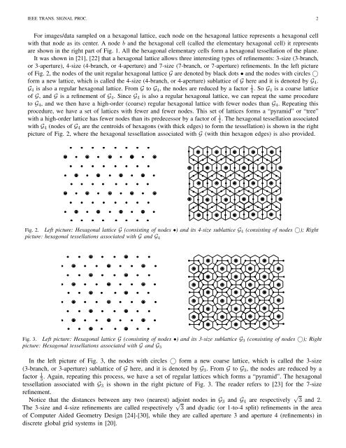In the left picture of Fig. 2, the nodes of the unit regular hexagonal lattice G are denoted by black dots • and the nodes with circles ○ form a new lattice, which is called the 4-size (4-branch, or 4-aperture) sublattice of G here and it is denoted by G 4 . G 4 is also a regular hexagonal lattice. From G to G 4 , the nodes are reduced by a factor 1 4 . So G 4 is a coarse lattice of G, and G is a refinement of G 4 . Since G 4 is also a regular hexagonal lattice, we can repeat the same procedure to G 4 , and we then have a high-order (coarse) regular hexagonal lattice with fewer nodes than G 4 . Repeating this procedure, we have a set of lattices with fewer and fewer nodes. This set of lattices forms a “pyramid” or “tree” with a high-order lattice has fewer nodes than its predecessor by a factor of 1 4 . The hexagonal tessellation associated with G 4 (nodes of G 4 are the centroids of hexagons (with thick edges) to form the tessellation) is shown in the right picture of Fig. 2, where the hexagonal tessellation associated with G (with thin hexagon edges) is also provided. Fig. 2. Left picture: Hexagonal lattice G (consisting of nodes •) and its 4-size sublattice G 4 (consisting of nodes ○); Right picture: hexagonal tessellations associated with G and G 4 Fig. 3. Left picture: Hexagonal lattice G (consisting of nodes •) and its 3-size sublattice G 3 (consisting of nodes ○); Right picture: Hexagonal tessellations associated with G and G 3 In the left picture of Fig. 3, the nodes with circles ○ form a new coarse lattice, which is called the 3-size (3-branch, or 3-aperture) sublattice of G here, and it is denoted by G 3 . From G to G 3 , the nodes are reduced by a factor 1 3 . Again, repeating this process, we have a set of regular lattices which forms a “pyramid”. The hexagonal tessellation associated with G 3 is shown in the right picture of Fig. 3. The reader refers to [23] for the 7-size refinement. Notice that the distances between any two (nearest) adjoint nodes in G 3 and G 4 are respectively √ 3 and 2. The 3-size and 4-size refinements are called respectively √ 3 and dyadic (or 1-to-4 split) refinements in the area of Computer Aided Geometry Design [24]-[30], while they are called aperture 3 and aperture 4 (refinements) in discrete global grid systems in [20].
IEEE TRANS. SIGNAL PROC. 3 The refinements of the hexagonal lattice allow the multiresolution (multiscale) analysis method to be used to process hexagonally sampled data. The dyadic (4-size) refinement is the most commonly used refinement for multiresolution image processing, and there are many papers on the construction and/or applications of dyadic hexagonal filter banks and wavelets, see e.g. [11], [12], [18], [31]-[37]. Though √ 7-refinement (7-size refinement) has some special properties, the √ 7-refinement multiresolution data processing results in a reduction in resolution by a factor 7 which may be too coarse and is undesirable. The reader refers to [23] for the construction of √ 7- refinement wavelets. The √ 3 (3-size) refinement is the most appealing refinement for multiresolution data processing due to the fact that √ 3-refinement generates more resolutions and, hence, it gives applications more resolutions from which to choose. This fact is the main motivation for the study of √ 3-refinement subdivision in [24]-[30] and it is also the main reason for the recommendation to use the √ 3-refinement for discrete global grid systems in [20], where √ 3-refinement is called 3 aperture. The √ 3-refinement has been used by engineers and scientists of the PYXIS innovation Inc. to develop The PYXIS Digital Earth Reference Model [38]. However, there is little work on √ 3- refinement wavelets. [40], [41] are the only articles available in the literature on this topic. (The readers to [39] for rotation covariant quincunx wavelets on square lattice.) The authors of [41] construct biorthogonal √ 3-refinement wavelets by adopting the method in [35] for the construction of dyadic wavelets. The wavelets in [35] and [41] are constructed for the purpose of surface multiresolution processing which involves both regular and extraordinary nodes (vertices) in the surfaces. It is hard to calculate the L 2 inner product of the scaling functions (also called basis functions) and wavelets associated with extraordinary nodes. Thus, when considering the biorthogonality, [35] and [41] do not use the L 2 inner product. Instead, they use a “discrete inner product” related to the discrete filters. That discrete inner product may result in basis functions and wavelets which are not L 2 (IR 2 ) functions. Indeed, the √ 3-refinement analysis basis functions and wavelets (even associated with regular nodes) constructed in [41] are not in L 2 (IR 2 ), and hence they cannot generate Riesz bases for L 2 (IR 2 ). In this paper we study the construction of orthogonal and biorthogonal √ 3-refinement wavelets (for regular nodes) with the conventional L 2 inner product. The rest of this paper is organized as follows. In Section II, we provide √ 3-refinement multiresolution decomposition and reconstruction algorithms and some basic results on the orthogonality/biorthogonality of √ 3-refinement filter banks. In Section III, we study the construction of orthogonal √ 3-refinement wavelets. We will present a block structure of orthogonal FIR filter banks. In Section IV, we address the construction of √ 3-refinement perfect reconstruction (biorthogonal) filter banks with 6-fold axial symmetry and the associated biorthogonal wavelets. In this paper we use bold-faced letters such as k, x, ω to denote elements of Z 2 and IR 2 . A multi-index k of Z 2 and a point x in IR 2 will be written as row vectors k = (k 1 , k 2 ), x = (x 1 , x 2 ). However, k and x should be understood as column vectors [k 1 , k 2 ] T and [x 1 , x 2 ] T when we consider Ak and Ax, where A is a 2×2 matrix. For a matrix M, we use M ∗ to denote its conjugate transpose M T , and for a nonsingular matrix M, M −T denotes (M −1 ) T . II. MULTIRESOLUTION PROCESSING WITH √ 3-REFINEMENT FILTER BANKS In this section, we provide √ 3-refinement multiresolution decomposition and reconstruction algorithms and present some basic results on the orthogonality/biorthogonality of √ 3-refinement filter banks. A. √ 3-refinement multiresolution algorithms Let G denote the regular unit hexagonal lattice defined by where G = {k 1 v 1 + k 2 v 2 : k 1 , k 2 ∈ Z}, (1) v 1 = [1, 0] T , v 2 = [− 1 2 , √ 3 2 ]T . To a node g = k 1 v 1 +k 2 v 2 of G, we use (k 1 , k 2 ) to indicate g, see the left part of Fig. 4 for the labelling of G. Thus, for hexagonal data c sampled on G, instead of using c g , we use c k1 ,k 2 to denote the pixel of c at g = k 1 v 1 + k 2 v 2 .
Page 1: IEEE TRANS. SIGNAL PROC. 1 Orthogon
Page 5 and 6: IEEE TRANS. SIGNAL PROC. 5 b1 f 2 c
Page 7 and 8: IEEE TRANS. SIGNAL PROC. 7 S 0 S 0"
Page 9 and 10: IEEE TRANS. SIGNAL PROC. 9 where I
Page 11 and 12: IEEE TRANS. SIGNAL PROC. 11 Fig. 9.
Page 13 and 14: IEEE TRANS. SIGNAL PROC. 13 which i
Page 15 and 16: IEEE TRANS. SIGNAL PROC. 15 where
Page 17 and 18: IEEE TRANS. SIGNAL PROC. 17 10 1 0.
Page 19 and 20: IEEE TRANS. SIGNAL PROC. 19 and ⎡
Page 21 and 22: IEEE TRANS. SIGNAL PROC. 21 [28] P.

here - UMSL : Mathematics and Computer Science - University of ...

Create successful ePaper yourself

Delete template?

Save as template?