here - UMSL : Mathematics and Computer Science - University of ...
here - UMSL : Mathematics and Computer Science - University of ...
here - UMSL : Mathematics and Computer Science - University of ...

You also want an ePaper? Increase the reach of your titles
YUMPU automatically turns print PDFs into web optimized ePapers that Google loves.
IEEE TRANS. SIGNAL PROC. 4<br />
02 12<br />
22<br />
−11 01 11 21<br />
v 2<br />
00<br />
−20 −10 v 1 10 20<br />
−2−1 −1−1 0−1 1−1<br />
−2−2<br />
−1−2<br />
0−2<br />
c<br />
−20<br />
c<br />
12<br />
22<br />
c −11 01 c11<br />
c21<br />
c<br />
c −2−1<br />
c 02<br />
c<br />
−10<br />
c<br />
−2−2<br />
−1−1<br />
c<br />
c<br />
c<br />
00<br />
c<br />
−1−2<br />
0−1<br />
c<br />
c<br />
c<br />
10<br />
0−2<br />
c<br />
c 1−1<br />
20<br />
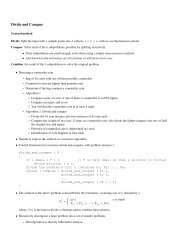
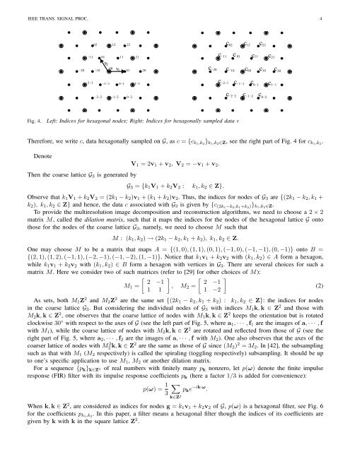
Fig. 4.<br />
Left: Indices for hexagonal nodes; Right: Indices for hexagonally sampled data c<br />
T<strong>here</strong>fore, we write c, data hexagonally sampled on G, as c = {c k1,k 2<br />
} k1,k 2∈Z, see the right part <strong>of</strong> Fig. 4 for c k1,k 2<br />
.<br />
Denote<br />
Then the coarse lattice G 3 is generated by<br />
V 1 = 2v 1 + v 2 , V 2 = −v 1 + v 2 .<br />
G 3 = {k 1 V 1 + k 2 V 2 :<br />
k 1 , k 2 ∈ Z}.<br />
Observe that k 1 V 1 + k 2 V 2 = (2k 1 − k 2 )v 1 + (k 1 + k 2 )v 2 . Thus, the indices for nodes <strong>of</strong> G 3 are {(2k 1 − k 2 , k 1 +<br />
k 2 ), k 1 , k 2 ∈ Z} <strong>and</strong> hence, the data c associated with G 3 is given by {c (2k1−k 2,k 1+k 2)} k1,k 2∈Z.<br />
To provide the multiresolution image decomposition <strong>and</strong> reconstruction algorithms, we need to choose a 2 × 2<br />
matrix M, called the dilation matrix, such that it maps the indices for the nodes <strong>of</strong> the hexagonal lattice G onto<br />
those for the nodes <strong>of</strong> the coarse lattice G 3 , namely, we need to choose M such that<br />
M : (k 1 , k 2 ) → (2k 1 − k 2 , k 1 + k 2 ), k 1 , k 2 ∈ Z.<br />
One may choose M to be a matrix that maps A = {(1, 0), (1, 1), (0, 1), (−1, 0), (−1, −1), (0, −1)} onto B =<br />
{(2, 1), (1, 2), (−1, 1), (−2, −1), (−1, −2), (1, −1)}. Notice that k 1 v 1 + k 2 v 2 with (k 1 , k 2 ) ∈ A form a hexagon,<br />
while k 1 v 1 + k 2 v 2 with (k 1 , k 2 ) ∈ B form a hexagon with vertices in G 3 . T<strong>here</strong> are several choices for such a<br />
matrix M. Here we consider two <strong>of</strong> such matrices (refer to [29] for other choices <strong>of</strong> M):<br />
[ ] [ ]<br />
2 −1<br />
2 −1<br />
M 1 =<br />
, M<br />
1 1<br />
2 =<br />
(2)<br />
1 −2<br />
As sets, both M 1 Z 2 <strong>and</strong> M 2 Z 2 are the same set {(2k 1 − k 2 , k 1 + k 2 ) : k 1 , k 2 ∈ Z}: the indices for nodes<br />
in the coarse lattice G 3 . But considering the individual nodes <strong>of</strong> G 3 with indices M 1 k, k ∈ Z 2 <strong>and</strong> those with<br />
M 2 k, k ∈ Z 2 , one observes that the coarse lattice <strong>of</strong> nodes with M 1 k, k ∈ Z 2 keeps the orientation but is rotated<br />
clockwise 30 ◦ with respect to the axes <strong>of</strong> G (see the left part <strong>of</strong> Fig. 5, w<strong>here</strong> a 1 , · · · , f 1 are the images <strong>of</strong> a, · · · , f<br />
with M 1 ), while the coarse lattice <strong>of</strong> nodes with M 2 k, k ∈ Z 2 are rotated <strong>and</strong> reflected from those <strong>of</strong> G (see the<br />
right part <strong>of</strong> Fig. 5, w<strong>here</strong> a 2 , · · · , f 2 are the images <strong>of</strong> a, · · · , f with M 2 ). One also observes that the axes <strong>of</strong> the<br />
coarser lattice <strong>of</strong> nodes with M2 2k, k ∈ Z2 are the same as those <strong>of</strong> G since (M 2 ) 2 = 3I 2 . In [42], the subsampling<br />
such as that with M 1 (M 2 respectively) is called the spiraling (toggling respectively) subsampling. It should be up<br />
to one’s specific application to use M 1 , M 2 or another dilation matrix.<br />
For a sequence {p k } k∈Z<br />
2 <strong>of</strong> real numbers with finitely many p k nonzero, let p(ω) denote the finite impulse<br />
response (FIR) filter with its impulse response coefficients p k (<strong>here</strong> a factor 1/3 is added for convenience):<br />
p(ω) = 1 ∑<br />
p k e −ik·ω .<br />
3<br />
k∈Z 2<br />
When k, k ∈ Z 2 , are considered as indices for nodes g = k 1 v 1 + k 2 v 2 <strong>of</strong> G, p(ω) is a hexagonal filter, see Fig. 6<br />
for the coefficients p k1,k 2<br />
. In this paper, a filter means a hexagonal filter though the indices <strong>of</strong> its coefficients are<br />
given by k with k in the square lattice Z 2 .