here - UMSL : Mathematics and Computer Science - University of ...

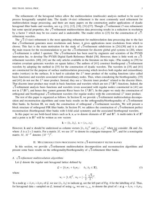
IEEE TRANS. SIGNAL PROC. 3
The refinements of the hexagonal lattice allow the multiresolution (multiscale) analysis method to be used to
process hexagonally sampled data. The dyadic (4-size) refinement is the most commonly used refinement for
multiresolution image processing, and there are many papers on the construction and/or applications of dyadic
hexagonal filter banks and wavelets, see e.g. [11], [12], [18], [31]-[37]. Though √ 7-refinement (7-size refinement)
has some special properties, the √ 7-refinement multiresolution data processing results in a reduction in resolution
by a factor 7 which may be too coarse and is undesirable. The reader refers to [23] for the construction of √ 7-
refinement wavelets.
The √ 3 (3-size) refinement is the most appealing refinement for multiresolution data processing due to the fact
that √ 3-refinement generates more resolutions and, hence, it gives applications more resolutions from which to
choose. This fact is the main motivation for the study of √ 3-refinement subdivision in [24]-[30] and it is also
the main reason for the recommendation to use the √ 3-refinement for discrete global grid systems in [20], where
√
3-refinement is called 3 aperture. The
√
3-refinement has been used by engineers and scientists of the PYXIS
innovation Inc. to develop The PYXIS Digital Earth Reference Model [38]. However, there is little work on √ 3-
refinement wavelets. [40], [41] are the only articles available in the literature on this topic. (The readers to [39] for
rotation covariant quincunx wavelets on square lattice.) The authors of [41] construct biorthogonal √ 3-refinement
wavelets by adopting the method in [35] for the construction of dyadic wavelets. The wavelets in [35] and [41]
are constructed for the purpose of surface multiresolution processing which involves both regular and extraordinary
nodes (vertices) in the surfaces. It is hard to calculate the L 2 inner product of the scaling functions (also called
basis functions) and wavelets associated with extraordinary nodes. Thus, when considering the biorthogonality, [35]
and [41] do not use the L 2 inner product. Instead, they use a “discrete inner product” related to the discrete filters.
That discrete inner product may result in basis functions and wavelets which are not L 2 (IR 2 ) functions. Indeed, the
√
3-refinement analysis basis functions and wavelets (even associated with regular nodes) constructed in [41] are
not in L 2 (IR 2 ), and hence they cannot generate Riesz bases for L 2 (IR 2 ). In this paper we study the construction of
orthogonal and biorthogonal √ 3-refinement wavelets (for regular nodes) with the conventional L 2 inner product.
The rest of this paper is organized as follows. In Section II, we provide √ 3-refinement multiresolution decomposition
and reconstruction algorithms and some basic results on the orthogonality/biorthogonality of √ 3-refinement
filter banks. In Section III, we study the construction of orthogonal √ 3-refinement wavelets. We will present a
block structure of orthogonal FIR filter banks. In Section IV, we address the construction of √ 3-refinement perfect
reconstruction (biorthogonal) filter banks with 6-fold axial symmetry and the associated biorthogonal wavelets.
In this paper we use bold-faced letters such as k, x, ω to denote elements of Z 2 and IR 2 . A multi-index k of Z 2
and a point x in IR 2 will be written as row vectors
k = (k 1 , k 2 ), x = (x 1 , x 2 ).
However, k and x should be understood as column vectors [k 1 , k 2 ] T and [x 1 , x 2 ] T when we consider Ak and Ax,
where A is a 2×2 matrix. For a matrix M, we use M ∗ to denote its conjugate transpose M T , and for a nonsingular
matrix M, M −T denotes (M −1 ) T .
II. MULTIRESOLUTION PROCESSING WITH
√
3-REFINEMENT FILTER BANKS
In this section, we provide √ 3-refinement multiresolution decomposition and reconstruction algorithms and
present some basic results on the orthogonality/biorthogonality of √ 3-refinement filter banks.
A. √ 3-refinement multiresolution algorithms
Let G denote the regular unit hexagonal lattice defined by
where
G = {k 1 v 1 + k 2 v 2 : k 1 , k 2 ∈ Z}, (1)
v 1 = [1, 0] T , v 2 = [− 1 2 , √
3
2 ]T .
To a node g = k 1 v 1 +k 2 v 2 of G, we use (k 1 , k 2 ) to indicate g, see the left part of Fig. 4 for the labelling of G. Thus,
for hexagonal data c sampled on G, instead of using c g , we use c k1 ,k 2
to denote the pixel of c at g = k 1 v 1 + k 2 v 2 .