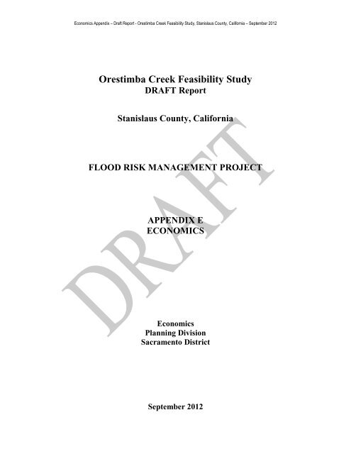
Orestimba Creek Feasibility Study - Stanislaus County

Economics Appendix – Draft Report - Orestimba Creek Feasibility Study, Stanislaus County, California – September 2012 

Orestimba Creek Feasibility Study 

DRAFT Report 

Stanislaus County, California 

FLOOD RISK MANAGEMENT PROJECT 

APPENDIX E 

ECONOMICS 

Economics 

Planning Division 

Sacramento District 

September 2012


This page was left blank to facilitate two-sided photocopying.


Executive Summary – Economics – Orestimba Creek Feasibility Study 

ES.1 

Overview 

The study area is located in the southwestern portion of Stanislaus County, in what is referred to 

as the Newman Division by the U.S. Census Bureau (see Figure 1). Orestimba Creek stretches 

approximately 7.5 within the study after having left the foothills of the Diablo Mountain Range. 

It is estimated that in the 500-year flood event the floodplain would encompass approximately 

20,000 acres, including the City of Newman (see Error! Reference source not found.). The 

City of Newman is the home of approximately 12,321 residents (2010 Census data). The study 

area is home to some of California’s most efficient and important agricultural industries. 

Tomato and vegetable processing, cheese manufacturing, and turkey hatching are examples of 

some of the agricultural industries located in the area. The area is acknowledged for crop 

diversity and productivity, which can be accredited to a combination of exceptional factors such 

as, soil quality, air quality, climate, and water supply. 

The city of Newman has experienced 14 floods in the past 58 years (1954, 1955, 1957-1959, 

1963, 1968, 1969, 1978, 1980, 1983, 1986, 1995 and 1998). The major floods occurred in 6 out 

of the last 14 flooding events (1955, 1958, 1963, 1980, 1983, 1995 and 1998), with 1995 being 

the flood of record. These floods occurred along Orestimba Creek and affected both rural and 

urban land uses. The frequency of flooding in and around Newman is similar that which occurs 

on an average cycle of between 4 to 5 years. These flooding events have affected the same 

general areas each time except when there was a levee failure or similar occurrence that changed 

the location of flooding and the type of land uses that were adversely affected. 

ES.2 

Purpose and Scope of Economic Analysis 

The purpose of this report is to present the results of the economic analysis performed for the 

Feasibility Study of the Orestimba Creek Project. The report documents the existing condition 

within the study area and proposed alternative plans to improve flood risk management, and 

designate the National Economic Development (NED) Plan for purposes of estimating federal 

interest for Orestimba Creek. The report presents findings related to flood risk, potential flood 

damages and potential flood damage reduction benefits. 

This Economic Appendix is intended to: 

• Document the current hydrologic data used in the economic analysis for the Orestimba 

study area under both the without-project and with-project conditions 

• Document the current hydraulic floodplains and HEC-FDA hydraulic input data used in 

the economic analysis for the Orestimba under both the without-project and with-project 

conditions 

ES-i


• Document the economic methodologies, major assumptions, models, and data used in the 

economic analysis for Orestimba under both the without-project and with-project 

conditions 

• Document the economic damage/benefit categories considered in the economic analysis 

for Orestimba under both the without-project and with-project conditions 

• Document the results (detailed HEC-FDA output files and EAD/AEP results) of the 

HEC-FDA model runs for Orestimba under both the without-project and with-project 

conditions 

• Document the cost estimates used to perform the net benefit and benefit-to-cost analyses 

• Describe the approach used to perform the with-project benefits analysis and document 

the results of the net benefit and benefit-to-cost analyses used to determine plan 

optimization and feasibility 

ES-ii


Figure E- 1: Orestimba Study Area and Economic Impact Areas 

ES.3 

Structural Inventory 

The without-project damages and with-project benefits were based on potential damages to 

residential structures and contents, non-residential (commercial, industrial and public) structures 

and contents, automobiles, agriculture, cleanup costs and emergency. The study area was 

ES-iii


divided into two Economic Impact Areas for purposes of this analysis; Urban and Rural. The 

delineation of these impact areas can be found in Error! Reference source not found.. 

There are approximately 1365 structures in the Orestimba study area within the 0.2% (1/500) 

Annual Chance Exceedance (ACE) floodplain boundary. The 0.2% annual chance floodplain is 

shown in Figure E- 2. Structure counts are presented in Table E- 1. Total value of damageable 

property (structures and contents) is displayed in Table E- 2 and is approximately $300 million. 

Table E- 1: Structural Inventory 

Number of Units within the 0.2% (1/500) Annual Chance Floodplain by Land Use 

Economic 

Impact Area 

Residential Commercial Industrial Public Total 

Rural 158 0 0 0 158 

Urban 1122 62 16 7 1207 

TOTAL 1,280 62 16 7 1365 

Table E- 2: Value of Damageable Property 

Within the 0.2% (1/500) Annual Chance Floodplain 

October 2011 Prices ($1,000’s) 

Land Use 

Structural Value 

Content Value 

Rural Urban Rural Urban 

TOTAL 

Residential 17,706 123,204 8,853 61,602 $211,365 

Commercial 0 23,732 0 25,030 $48,763 

Industrial 0 13,593 0 20,014 $33,607 

Public 0 4,541 0 2,123 $6,664 

TOTAL $17,706 $165,070 $8,853 $108,769 $300,398 

ES-iv


Figure E- 2: Existing Condition 0.2% (1/500) Annual Chance Floodplain 

ES-v


ES.4 

Without Project Damages 

To find the damage for any given flood frequency, the discharge for that frequency is first 

located in the discharge-frequency graph (graph #1), then the river channel stage associated with 

that discharge value is determined in the stage-discharge graph (graph #2). Once the levees fail 

and water enters the floodplain, the stages (water depths) in the floodplain inundate structures 

and cause damage (graph #4, left side). By plotting this damage and repeating for process many 

times, the damage-frequency curve is determined (graph #4, right side). EAD is then computed 

by finding the area under the flood damage-frequency curve by integration for the without, 

interim, and with project conditions. Reductions in EAD attributable to projects are flood 

reduction benefits. Uncertainties are present for each of the functions discussed above and these 

are carried forth from one graph to the next, ultimately accumulating in the EAD. These 

uncertainties are shown in Figure E- 3 as “error bands” located above and below the hydrologic, 

hydraulic and economics curves. 

Figure E- 3: Uncertainty in Discharge, Stage and Damage 

in Determination of Expected Annual Damages 

Single-event damages for the 20%, 10%, 5%, 2%, 1%, 0.5% and 0.2% ACE event flood events 

were computed in the economic model (HEC-FDA v1.2.5a) and are presented in Table E- 3. 

These results represent probability damages prior to the application of economic uncertainty 

parameters. 

ES-vi


Table E- 3: Without Project Probability-Stage-Damage Functions – by Economic Impact Area (EIA) 


Damage 

Category 

EIA Urban Rural Urban Rural Urban Rural Urban Rural Urban Rural Urban Rural Urban Rural Urban Rural 

AUTO $0 $0 $0 $101 $71 $170 $100 $210 $114 $266 $150 $301 $169 $339 $189 $392 

Clean $0 $0 $0 $66 $1,134 $132 $1,752 $167 $1,914 $200 $2,065 $229 $2,115 $251 $2,180 $281 

Emergency $0 $0 $0 $386 $364 $531 $930 $602 $1,101 $687 $1,416 $765 $1,521 $847 $1,627 $927 

Commercial $0 $0 $39 $0 $2,266 $0 $3,210 $0 $3,386 $0 $3,699 $0 $3,798 $0 $3,919 $0 

Industrial $0 $0 $0 $0 $2,232 $0 $2,414 $0 $2,476 $0 $2,547 $0 $2,586 $0 $2,685 $0 

Public $0 $0 $0 $0 $78 $0 $142 $0 $151 $0 $177 $0 $182 $0 $189 $0 

Residential $0 $0 $43 $782 $5,115 $1,798 $12,001 $2,381 $13,818 $3,001 $15,952 $3,511 $16,589 $3,967 $17,334 $4,583 

Agricultural $0 $0 $0 $3,190 $0 $5,877 $0 $7,377 $0 $8,698 $0 $9,539 $0 $10,267 $0 $11,025 

Subtotals $0 $0 $82 $4,525 $11,260 $8,508 $20,549 $10,737 $22,960 $12,853 $26,005 $14,346 $26,959 $15,670 $28,124 $17,207 

TOTAL 

99% (1/1) 20% (1/5) 10% (1/10) 5% (1/20) 

Annual Chance Exceedance Probability of Event and Damages 

2% (1/50) 1% (1/100) 0.5% (1/200) 0.2% (1/500) 

$0 $4,607 $19,767 $31,286 $35,813 $40,351 $42,630 $45,332 

ES-vii


The HEC-FDA model results (Expected Annual Damages) for contents, structures, automobiles, 

cleanup costs and emergency costs for each economic impact area (EIA) under the without 

project condition from are found in Table E- 4. Total study area without project expected annual 

damages are equal to approximately $5.4 million. 

Table E- 4: Expected Annual Damages - Without Project Conditions 


Damage EAD by Impact Area 

Category Rural Urban 

TOTAL 

Agriculture $1,381 $0 $1,381 

Auto $61 $50 $111 

Cleanup $37 $183 $220 

Emergency $148 $194 $341 

Commercial $0 $520 $520 

Industrial $0 $417 $417 

Public $0 $33 $33 

Residential $657 $1,733 $2,389 

TOTAL $2,284 $3,130 $5,413 

ES.5 

With-Project Damages and Benefits 

This section will describe how benefits of flood damage reduction of the final array of 

alternatives were estimated. Non-monetary outputs such as environmental measures, which may 

vary for the final array of alternatives, are not included but may factor in the plan formulation 

decision process. 

Benefits were determined by incorporating residual with-project floodplains and rating curves 

into the FDA model that represent various with project improvements. Flood risk management 

benefits equal the difference between the without project damage conditions and the with-project 

residual damages. 

The reduction in project flood plains in both extent and depth from the larger without project 

flood plains accounts for the decrease in damages of the given alternative. 

Optimization of Chevron Levee Height 

The chevron levee height was optimized by inserting incrementally higher levees into HEC-FDA 

and comparing the increased benefits to the estimated incremental costs. Costs were estimated 

by Cost Engineering for a levee equal to the mean 2% (1/50) WSEL and the mean 0.5% (1/200) 

WSEL + 3ft. These two values were then used to create a linear interpolation between the two 

points in order to estimate the cost of incrementally higher levees. These costs include only 

ES-viii


those costs that are variable depending on the height of the levee (mostly fill material). The 

index point used for this height optimization was at the Stuhr Rd. and CCID canal intersection, 

so the benefits here appear higher than those reported in the without project chapter of this 

report. The optimization of the levee height must use an index point at a location where the 

levee would be located to come up with a proper levee elevation. The particular index point 

location for the optimization was chosen because it was the first point that flooding overtopped 

the existing CCID canal (near Stuhr Rd), which is adjacent to the chevron levee’s location. This 

was the original location for the economic evaluation as well, but the index was changed later 

based on rating curve sensitivity for high probability events (see section 5.5 of the main 

Economic Appendix) and likely overestimation of EAD. Because the CCID Canal location and 

the eventual urban economic analysis index location (intersection of Lundy Rd. and the Railroad) 

have rating curves with nearly identical slopes for lower probability events (2% (1/50) annual 

chance event and above), the difference in an optimization height was assumed negligible. To 

confirm this assumption, a sensitivity analysis was performed using the Lundy Rd. index 

location and the optimal heights were found to be within 0.2 ft of each other and well within 

error bands in stage/ground elevations. The final benefits used for economic justification will be 

based on the without project conditions as summarized in Table E- 6. In addition, costs reported 

here do not reflect Total Project First Costs; instead these costs represent only those variable 

costs in relation to levee height. Total Project First Costs can be found in Table E- 10. This 

analysis is solely used for optimization of the levee height in order for costs and residual benefits 

to be determined in more detail on only one plan. As shown in Table E- 5 below, the optimal 

elevation for the top of levee at this index point is determined to be around 112.75 feet, which 

equates to a levee 5.5 to 8 feet tall depending on the ground elevation changes along the levee 

alignment. It is noted here that this height is higher than the mean 0.2% (1/500) WSEL, but 

because of the alluvial fan type of flooding, the mean 0.2% (1/500) WSEL is only 9 inches 

higher than the mean 2% (1/50) mean WSEL. 

ES-ix


Table E- 5: Optimization of the Chevron Levee Height at Stuhr Rd and CCID Canal 

Crossing 

Return 

Period 

Levee 

Elevation (ft.) 

*Annual Benefits 

($1,000's) 

*Annual Costs 

($1,000's) 

*Net Benefits 

($1,000's) 

1/50 111.21 6,079 749 5,330 

111.25 6,188 753 5,435 

111.5 6,412 777 5,636 

111.75 6,612 800 5,812 

1/500 112 6,785 823 5,962 

112.25 6,910 847 6,063 

112.5 6,990 870 6,120 

112.75 7,035 893 6,142 

113 7,056 917 6,139 

113.25 7,064 940 6,124 

113.5 7,066 964 6,103 

113.75 7,067 987 6,080 

114 7,067 1,010 6,057 

114.25 7,067 1,034 6,034 

1/200+3ft 114.8 7,067 1,085 5,982 

* The Benefits and Costs shown here are different than those presented in Chapter 3 of the main report, 

because these show the actual values used for the sensitivity, while the main report has adjusted those 

values to reflect total project benefits and costs. Annual Benefits, Annual Costs and Net Benefits shown 

here do not reflect actual benefits and total costs used for final net benefit and BCR calculations. The 

index point used for this height optimization exercise is different from the one used for economic 

justification. Benefits and costs used for economic justification can be found in Table E- 10. More 

information about different index points and the effect on damages in this study area is available upon 

request. 

Sensitivity analysis was performed on other index locations along the levee alignment and the 

results were within 0.2ft, which is well within the error bands of the ground elevations. The 

optimized height is approximately 1.5ft above the existing 2% (1/50) WSEL, which is reasonable 

for an alluvial fan floodplain given uncertainty in ground elevations and stages. 

ES-x


The Final Array of Alternatives 

The final array of alternatives is listed below. See the main report for a detailed description of 

all other alternatives that were evaluated and screened out during the plan formulation process. 

1. No Action Plan 

2. Chevron Levee: Chevron levee at optimized height. (TOL elevation of 112.75 feet) 

3. Local Plan: Chevron Levee set at a height equal to the mean 0.5% (1/200) WSEL + 3 

Feet. (TOL elevation of 114.8 feet) 1 . 

A map showing the locations for the chevron levee is shown in Figure E- 4 below. For a more 

detailed description of these alternatives, please see the main report. 

Annual Benefits 

The mean annual benefits for the final 3 alternatives can be found in Table E- 6 below. Note that 

there is no incremental benefit for the Local Plan because the incrementally higher levee height 

does not provide an additional measurable benefit to the city of Newman and is mainly just to 

comply with State of California requirements. 

Residual Damage in the Urban EIA with the Chevron Levee in place consist of existing storm 

drainage damages caused by rain events above a 10% annual chance frequency. 

1 Senate Bill 5 (SB-5) in the State of California requires that levee’s be built to the mean 0.5% (1/200) annual 

chance exceedance event WSEL in order to qualify for state participation. 

ES-xi


Figure E- 4: Location of the Chevron Levee 

*Note: The Channel Modifications increment was screened out prior to the final array of alternatives. See the main 

report for more detail. 

Table E- 6: Annual Benefits – The Final Array – TOTAL Study Area 

October 2011 Prices ($1,000’s), 4% Interest Rate 

Alternative Annual Damages Annual Benefits Incremental Benefits 

1. No Action 5,413 0 0 

2. Chevron Levee at 

112.75ft 


114.8ft 

2,285 3,128 3,128 

2,285 3,128 0 

ES-xii


Probability Distribution of Damages Reduced 

In accordance with ER 1105-2-101, flood damages reduced were determined as mean values and 

by probability exceeded. The tables below show the benefits for each alternative for the 75%, 

50% and 25% probability that benefit exceeds indicated value. The damage reduced column 

represents the mean benefits for each increment and the 75%, 50% and 25% represent the 

probability that the flood damage reduction benefits exceed the number in that column for that 

increment. For example, Alternative 2, the Chevron Levee, has an average (mean) benefit of 

$3.1 million, but a 50% chance that benefits will be greater than $$2.7 million, 75% confidence 

that benefits will be equal or greater than $1.3 million and 25% confidence that benefits will 

exceed $4.4 million. This range is the probability distribution of damages reduced and 

represents the uncertainty in the benefit estimates and incorporates all the uncertainties in 

hydrology, hydraulics, and economics in the HEC-FDA model. The uncertainty in damages 

reduced should be considered when selecting an optimal plan during the plan formulation 

process. Judgment should be used to determine if an alternative meets a reasonable level of 

confidence regarding positive net benefits and identifying if changes in net benefits from 

alternative to alternative are significant. 

Table E- 7: Probability Distribution of Damages Reduced – TOTAL Study Area 


Alternative 

Without 

Project 

Annual Damage 

With 

Project 

Damage 

Reduced 

Probability Damage Reduced 

Exceeds Indicated Values 

75% 50% 25% 

1. No Action 5,413 5,413 0 0 0 0 


112.75ft 


114.8ft 

5,413 2,285 3,128 1,282 2,679 4,363 

5,413 2,285 3,128 1,282 2,679 4,363 

ES.6 

Project Performance 

In addition to damages estimates, HEC-FDA reports flood risk in terms of project performance. 

Three statistical measures are provided, in accordance with ER 1105-2-101, to describe 

performance risk in probabilistic terms. These include annual exceedance probability, long-term 

risk, and assurance by event. 

 

Annual exceedance probability measures the chance of having a damaging flood in any 

given year. 

ES-xiii


 

 

Long-term risk provides the probability of having one or more damaging floods over a 

period of time. 

Assurance is the probability that a target stage will not be exceeded during the 

occurrence of a specified flood. 

Project performance statistics for each impact area is displayed by impact area for both without 

and with project conditions in the tables below. 

Table E- 8: Project Performance – With Project Conditions – Rural EIA 

Alternative 

Annual 

Exceedance 

Probability 

Median 

Expected 

10 Year 

Period 

Long-Term Risk 

30 Year 

Period 

50 Year 

Period 

Assurance by Events 

10% 2% 1% 0.20% 

1. No Action 24.31% 24.22% 94% 99% 99% 6% 2% 1% 1% 


112.75ft 


114.8ft 

24.31% 24.22% 94% 99% 99% 6% 2% 1% 1% 

24.31% 24.22% 94% 99% 99% 6% 2% 1% 1% 

Table E- 9: Project Performance – With Project Conditions – Urban EIA 

Alternative 

Annual 

Exceedance 

Probability 

Median 

Expected 

10 Year 

Period 


30 Year 

Period 

50 Year 

Period 


10% 2% 1% 0.20% 

1. No Action 14.43% 15.13% 81% 98% 99% 13% 0% 0% 0% 


112.75ft 


114.8ft 

0.01% 0.04% 0% 1% 2% 99% 99% 99% 98% 

0.00% 0.00% 0% 0% 0% 99% 99% 99% 99% 

ES.7 

Net Benefit Analysis 

With benefits calculations complete, annual costs need to be derived to complete the benefit cost 

analysis. Economic feasibility and project efficiency are determined through benefit cost 

analysis. For a project or increment to be feasible, benefits must exceed costs and the most 

efficient alternative is the one that maximizes net benefits (annual benefits minus annual costs). 

ES-xiv


The NED Plan 

With the Channel Modifications increment dropping from the Federal Interest, the optimized 

Chevron Levee becomes the NED Plan. 

The Tentatively Recommended Plan 

The only difference between the Tentatively Recommended Plan and the NED Plan is the height 

of the chevron levee. The height of the chevron levee for the local plan must meet State of 

California requirements of being at least 3 feet above the with-project 200 year mean WSEL. 

This means a levee that is about 7.5 to 10 feet tall or approximately 2 feet taller than the federal 

interest levee. 

Benefits and Costs 

A more rigorous and detailed MCACES cost estimate was performed for the NED Chevron 

Levee and the LPP (Alternatives 2 and 3 respectively). Benefits and costs for these alternatives 

are provided in Table E- 10 below. 

ES-xv


Table E- 10: Total Annual Benefits and Costs by Alternative 


Based on a 50-year Period of Analysis 

FRM Costs/Benefits 

ITEM 

Tentatively Recommended 

Tentative NED Plan (Alt 2) 

Plan (Alt 3) 

Investment Costs: 

First Costs 35,219 44,056 

Less Cult Res (281) (353) 

Less Sunk PED costs 0 0 

Interest During Construction 2,141 2,679 

Total 37,079 46,382 

Annual Cost: 

Interest and Amortization 1,726 2,159 

OMRR&R 164 180 

Subtotal 1,890 2,339 

Annual Benefits: 3,128 3,128 

Net Annual FRM Benefits 1,238 789 

FRM Benefit-Cost Ratio 1.66 1.34 

ES.8 

Conclusions 

The NED Plan is Alternative 2, the stand-alone Chevron Levee at the optimized elevation of 

112.75 feet. The NED and it has an annual net benefit of $1.2 million and a BCR of 1.6. The 

Tentatively Recommended Plan is Alternative 3, the stand-alone Chevron Levee at an elevation 

of 114.8ft. The Recommended Plan has net annual benefits of $0.8 million and a BCR of 1.3. 

ES-xvi


ORESTIMBA CREEK PROJECT, CALIFORNIA 

FEASIBILITY STUDY AND REPORT 

ECONOMICS APPENDIX 

APPENDIX E 

Draft Report 

August 2012 

TABLE OF CONTENTS 

Executive Summary – Economics – Orestimba Creek Feasibility Study ..................... i 

ES.1 

ES.2 

ES.3 

ES.4 

ES.5 

ES.6 

ES.7 

ES.8 

Overview .............................................................................................................. i 

Purpose and Scope of Economic Analysis........................................................... i 

Structural Inventory ........................................................................................... iii 

Without Project Damages .................................................................................. vi 

With-Project Damages and Benefits ................................................................ viii 

Project Performance ......................................................................................... xiii 

Net Benefit Analysis ........................................................................................ xiv 

Conclusions ...................................................................................................... xvi 

1.0 Introduction ........................................................................................................... 1 

1.1 Purpose and Scope ............................................................................................ 1 

1.2 Study Area ......................................................................................................... 1 

1.3 History of Flooding ........................................................................................... 1 

1.4 Methodology (References and Methods Cited) .............................................. 3 

2.0 Flood Plain Area and Inventory .......................................................................... 4 

2.1 Economic Impact Areas ................................................................................... 4 

2.2 Inventory of Structures and Property in Study Area .................................... 5 

2.3 Value of Damageable Property- Structure Value .......................................... 9 

2.4 Value of Damageable Property- Content Value ............................................. 9 

3.0 Depth-Damage Relationships and Flooding Characteristics .......................... 13 

3.1 Determining Flood Depths ............................................................................. 13 

3.2 Depth-Damage Relationships ......................................................................... 13 

i


4.0 Uncertainty and Other Categories .................................................................... 16 

4.1 FLO-2D Grid Cells and Parcel Assignments using GIS.............................. 16 

4.2 Economic Uncertainty Parameters ............................................................... 16 

4.3 Other Damage Categories .............................................................................. 19 

5.0 Expected Annual Damages –Without Project Conditions .............................. 21 

5.1 HEC-FDA Model ............................................................................................ 21 

5.2 Estimation of Expected Annual Damages..................................................... 21 

5.3 Probability-Stage-Damage Functions ........................................................... 23 

5.3.1 Stage-damage curves and alluvial fan (FLO-2D) floodplain modeling ..... 25 

5.4 Existing Condition Expected Annual Damages ........................................... 26 

5.5 Effect of Risk and Uncertainty on Existing Condition Urban Expected 

Annual Damages in HEC-FDA .................................................................................. 26 

5.6 EAD Future Conditions and Equivalent Annual Damages ........................ 29 

5.7 Project Performance- Without Project Conditions ..................................... 29 

6.0 With Project Conditions –Flood Damage Reduction Benefits ........................ 31 

6.1 2009 Preliminary Incremental Alternatives Analysis .................................. 31 

6.1.1 Project Conditions- Model Simulations ........................................................ 32 

6.1.2 Average Annual Equivalent Damages –With Project Conditions .............. 32 

6.1.3 Alternatives Evaluated – Preliminary Screening Net Benefit Analysis ..... 32 

6.1.3.1 Alternatives Carried forward from Preliminary Screening for Further 

Evaluation .................................................................................................................... 34 

6.1.4 Optimization of the Chevron Levee Height .................................................. 35 

6.1.4.1 Sensitivity of Optimization Height to Index Location ................................. 36 

6.1.5 Incremental Analysis of the Channel Modifications ................................... 37 

6.2 The Final Array of Alternatives .................................................................... 37 

6.3 Annual Benefits for the Final Array of Alternatives ................................... 38 

6.4 Probability Distribution – Damages Reduced .............................................. 39 

6.5 Project Performance – With Project Conditions ......................................... 41 

6.6 Other Benefits.................................................................................................. 42 

7.0 Benefit-Cost Analysis .......................................................................................... 45 

7.1 Annual Costs.................................................................................................... 45 

ii


7.2 Net Benefits ...................................................................................................... 45 

7.2.1 The NED Plan .................................................................................................. 45 

7.2.2 The Tentatively Recommended Plan ............................................................ 45 

7.2.3 Benefits and Costs ........................................................................................... 45 

7.2.3.1 Net Benefits and BCR sensitivity to uncertainty .......................................... 46 

Attachment A: Without Project Hydrologic and Hydraulic Relationships ............. 49 

Attachment B: Agricultural Economic Analysis ......................................................... 52 

Attachment C: Regional Economic Development (RED)........................................... 77 

Attachment D: Other Social Effects (OSE) ................................................................. 88 

iii


List of Tables 

Table 2-1: Structural Inventory .................................................................................... 5 

Table 2-2: Content Values (Non-residential).............................................................. 11 

Table 2-3: Value of Damageable Property ................................................................. 12 

Table 3-1: Depth Damage Curves for Residential (Structure and Content) ........... 14 

Table 3-2: Depth Damage Curves for Non-Residential Structures .......................... 14 

Table 3-3: Depth Damage Curves for Non-Residential Content 1-story ................. 15 

Table 3-4: Depth Damage Curves for Non-Residential Content 2-story ................. 15 

Table 4-1: Standard Deviations for Risk and Uncertainty in Structure & Content 

Value ......................................................................................................................... 17 

Table 4-2: Standard Deviations for Depth-Damage Percentages - Residential ...... 17 

Table 4-3: Non-Residential Content Depth-Damage Uncertainty ............................ 18 

Table 4-4: Automobile Depth Damage Function ....................................................... 19 

Table 4-5: Emergency Costs Depth-Damage Curves ................................................ 20 

Table 4-6: Cleanup Cost Depth-Damage Curve ........................................................ 20 

Table 5-1: Without Project Probability-Stage-Damage Functions - Rural Impact 

Area .......................................................................................................................... 24 

Table 5-2: Without Project Probability-Stage-Damage Functions - Urban Impact 

Area .......................................................................................................................... 24 

Table 5-3: Without Project Probability-Stage-Damage Functions – TOTAL 

STUDY AREA ......................................................................................................... 25 

Table 5-4: Number of structures flooded by event – Urban EIA only ...................... 26 

Table 5-5: Expected Annual Damages - Without Project Conditions ..................... 26 

Table 5-6: Index Point Sensitivity Runs...................................................................... 29 

Table 5-7: Project Performance by EIA ..................................................................... 30 

Table 6-1: Preliminary Screening Annual Benefits and Costs by Alternative ........ 33 

Table 6-2: Optimization of the Chevron Levee height at Stuhr Rd and CCID Canal 

Crossing ................................................................................................................... 36 

Table 6-3: Incremental Benefits of Channel Modifications ....................................... 37 

iv


Table 6-4: Annual Benefits – The Final Array – Rural EIA .................................... 38 

Table 6-5: Annual Benefits – The Final Array – Urban EIA ................................... 39 

Table 6-6: Annual Benefits – The Final Array – TOTAL Study Area .................... 39 

Table 6-7: Probability Distribution of Damages Reduced – Rural EIA .................. 40 

Table 6-8: Probability Distribution of Damages Reduced – Urban EIA ................. 40 

Table 6-9: Probability Distribution of Damages Reduced – TOTAL Study Area .. 40 

Table 6-10: Project Performance – Rural EIA .......................................................... 42 

Table 6-11: Project Performance – Urban EIA ......................................................... 42 

Table 7-1: Total Annual Benefits and Costs by Alternative ..................................... 46 

Table 7-2: Net Benefits and Benefit-to-Cost Ratio Ranges – Final Array of 

Alternatives .............................................................................................................. 48 

v


List of Figures 

Figure 2-1: Orestimba Creek Economic Impact Areas ............................................... 4 

Figure 2-2: Orestimba Creek Existing Condition Floodplain - 10% (1/10) Annual 

Chance Event ............................................................................................................. 7 

Figure 2-3: Orestimba Creek Existing Condition Floodplain – 0.2% (1/500) Annual 

Chance Event ............................................................................................................. 8 

Figure 5-1: Uncertainty in Discharge, Stage and Damage ........................................ 22 

Figure 5-2: Index Locations (For Reporting and Sensitivity Runs) ......................... 28 

Figure 6-1: Location of the Chevron Levee and Channel Modifications ................ 34 

vi


1.0 Introduction 

1.1 Purpose and Scope 

The purpose of this report is to present the results of the economic analysis performed for the 

Feasibility Study of the Orestimba Creek Project. The report documents the existing condition 

within the study area and proposed alternative plans to improve flood risk management, and 

designate the National Economic Development (NED) Plan for purposes of estimating federal 

interest for Orestimba Creek. The report presents findings related to flood risk, potential flood 

damages and potential flood damage reduction benefits. 

1.2 Study Area 

The study area is located in the southwestern portion of Stanislaus County, in what is referred to 

as the Newman Division by the U.S. Census Bureau (see, Figure 1). Orestimba Creek stretches 

approximately 7.5 within the study after having left the foothills of the Diablo Mountain Range. 

It is estimated that in the 500-year flood event the floodplain would encompass approximately 

20,000 acres, including the City of Newman (see Figure 2-1). The City of Newman is the home 

of approximately 12,321 residents (2010 Census data). Newman is home to the world’s first 

school bus company and along with the surrounding area, it is home to some of California’s most 

efficient and important agricultural industries. Tomato and vegetable processing, cheese 

manufacturing, and turkey hatching are examples of some of the agricultural industries located in 

the area. The area is acknowledged for crop diversity and productivity, which can be accredited 

to a combination of exceptional factors such as, soil quality, air quality, climate, and water 

supply. 

1.3 History of Flooding 

The city of Newman has experienced 14 floods in the past 58 years (1954, 1955, 1957-1959, 

1963, 1968, 1969, 1978, 1980, 1983, 1986, 1995 and 1998). The major floods occurred in 6 out 

of the last 14 flooding events (1955, 1958, 1963, 1980, 1983, 1995 and 1998). These floods 

occurred along Orestimba Creek and affected both rural and urban land uses. The frequency of 

flooding in and around Newman is similar that which occurs on an average cycle of between 4 to 

5 years. These flooding events have affected the same general areas each time except when there 

was a levee failure or similar occurrence that changed the location of flooding and the type of 

land uses that were adversely affected. The following flooding summary descriptions focus on 

the seven largest major flooding events. 

In 1955, floodwaters inundated agricultural, residential, and commercial properties; caused 

breaks in the DMC; washed out public streets and culverts; inundated and closed public streets in 

many areas; and washed out the Southern Pacific Railroad ballast and ties. 

The April 1958 flood damaged agricultural lands and public facilities in the Orestimba Creek 

basin. Some residents were forced to evacuate their homes. Subsequently, in the 1959 flood, 

1


Orestimba Creek floodwaters eroded the west embankment of the Anderson Road bridge causing 

it to drop 2 feet in elevation and create several cracks in the bridge. 

In early February 1963, about 6 inches of rainfall over the Orestimba Creek basin caused both 

flooding and one of the largest peak flows of record. About 2,000 acres located 4 to 5 miles 

north of Newman were inundated by shallow floodwaters. Agricultural lands experienced soil 

erosion and silt deposition. The DMC siphon and access ramps to both road and railroad bridges 

were eroded to an extent that required repair. These floodwaters left debris that had to be 

removed. 

Extensive rainfall in January 1969 caused the flooding of nearly 2,000 acres. Flood damages 

occurred primarily on agricultural lands and consisted of erosion of agricultural soils, deposition 

of sediment, and prolonged field inundation which adversely affected area walnut orchards. 

In March 1995, Newman experienced the worst flood in the city's 107 year history. During the 

storm, the valley floor received between 2.5 and 4.0 inches of rain within 24-hours and more 

intense rainfall in the foothills. On March 10, 1995, the USGS gauging station located upstream 

from the California Aqueduct siphon registered a peak flow of 12,000 cfs. A convalescent 

hospital located on the north side of the city was entirely inundated by 2 feet of water in the 

building and 4 feet of water in the parking lot. Sixty-five residents were evacuated by a Medi- 

Flight helicopter after a failed attempt to use two ambulances and a school bus. Expansive areas 

of agricultural cropland were inundated by floodwaters. Additionally, a bean crop storage 

facility located just north of the city experienced extensive flooding affecting land and property 

forced the business into bankruptcy shortly after the flood. A neighboring agricultural packing 

facility also experienced flooding. 

During the 1995 flood event, many public streets and highways, including State Highway 33, 

were closed. These road closures limited or, in some cases, prevented access for emergency 

vehicles which resulted in diminished local and regional emergency response capabilities. 

Similar public health risks caused by area flooding included floodwater affected domestic water 

wells and individual septic systems, many of which were rendered unusable. 

In 1995, the city of Newman incurred reported flood damages of $7.8 million dollars (2011 

prices). Additionally, a bean crop storage facility located just north of the city experienced 

extensive flooding affecting land and property that loss of $465,000 dollars and was forced the 

business into bankruptcy shortly after the flood. This facility closure resulted in lost wages and 

income for 14 employees and 20 to 25 local growers. Another agricultural packing facility 

experienced $400,000 dollars in losses. Many public streets and highways including State 

Highway 33 were closed that limited or prevented access for emergency vehicles resulting in 

diminished emergency response capabilities. Flooding that affected domestic water wells and 

septic systems rendering many unusable also increased public health risks. 

Actual damages incurred from the 1998 flood are not known. 

The actual monetary cost of flood damages incurred by private property owners in West 

Stanislaus County during the most recent floods of record are difficult to fully assess. There are 

2


few written records on historical floods in the cities of Patterson and Newman and in the 

predominantly agricultural lands of Stanislaus County. Property owners have taken care of their 

own flood damages without assistance from the Federal Emergency Management Agency. 

Therefore, the historical record is not a good reference point for baseline economic damages. 

Due to the relatively shallow depths of flooding, sandbagging and other flood-fighting methods 

have also helped to truncate damages incurred. 

1.4 Methodology (References and Methods Cited) 

This economic analysis is in accordance with standards, procedures, and guidance of the U.S. 

Army Corps of Engineers. The Planning Guidance Notebook (ER 1105-2-100, April 2000) 

serves as the primary source for evaluation methods of flood risk management studies and was 

used as reference for this analysis. Additional guidance for risk-based analysis was obtained 

from EM 1110-2-1619, Engineering and Design – Risk-Based Analysis for Flood Damage 

Reduction Studies (August 1996) and ER 1105-2-101, Planning Risk-Based Analysis of 

Hydrology/Hydraulics, Geotechnical Stability, and Economics in Flood Damage Reduction 

Studies (March 1996). Economic evaluation was performed over a 50-year period of analysis. 

All values are presented in October 2011 price levels, and amortization calculations are based on 

the Fiscal Year 2012 federal discount rate of 4.0 percent as published in Corps of Engineers 

Economic Guidance Memorandum (EGM). 

3


2.0 Flood Plain Area and Inventory 

2.1 Economic Impact Areas 

For economic evaluation and project performance purposes, the study area was divided into two 

economic impact areas. Delineation was made to address differences in economic conditions 

and inventory type within the floodplain. A map showing the two impact areas (Rural and 

Urban) is shown in Figure 2-1. 

Figure 2-1: Orestimba Creek Economic Impact Areas 

4


2.2 Inventory of Structures and Property in Study Area 

A structural inventory was completed based on data gathered from assessor’s parcel data and onsite 

inspection of structures within the flood plain. Structures were determined to be within the 

economic study area by using Geographical Information Systems (GIS) to compare the 0.2% 

(1/500) ACE flood plain boundary (plus a buffer) with the spatially referenced assessor parcel 

numbers (APN). Information from the assessor’s parcel database (such as land use, building 

square footage, address) was supplemented during field visitation for each parcel within the 

flood plain by adding fields for foundation height, specific business activity (non-residential), 

building condition, type of construction, and number of units for example. Windshield survey 

field observation conducted on 100% of non-residential structures within 0.2% (1/500) ACE 

floodplain. Residential structures were sampled and grouped geographically by areas of 

homogeneous characteristics. Where square footage data was not available, the Google Earth 

measuring tool was used to estimate square footage. Parcels with structures, were categorized by 

land use and grouped into the following structural damage categories: 

1) Single Family Residential – includes all parcels represented by a single unit such 

as detached single family homes, individually owned condominiums and 

townhouses. 

2) Multiple Family Residential – includes residential parcels with more than one 

unit such as apartment complexes, duplexes and quadplex units. Each parcel may 

have multiple structures. 

3) Commercial – includes retail, office buildings, restaurants 

4) Industrial – includes warehouses, light and heavy manufacturing facilities. 

5) Public – includes both public and semi-public uses such as post office, fire dept, 

government buildings, schools and churches. 

6) Agriculture – Agricultural inventory was developed in a separate analysis. 

Please see Attachment B for a detailed writeup of this analysis. 

All parcels with structures were assigned to one of the listed categories. Some parcels have more 

than one physical structure and some structures, such as condominiums, are represented by 

multiple parcels. Table 2-1 displays the total number of structures within the 0.2% (1/500) ACE 

floodplain by category. Single family and Multi-family have been grouped together as 

“Residential” for presentation purposes. 

Table 2-1: Structural Inventory 

Number of Units within the 0.2% (1/500) Annual Chance Floodplain by Land Use 

Economic 

Impact Area 

Residential Commercial Industrial Public Total 

Rural 158 0 0 0 158 

Urban 1122 62 16 7 1207 

TOTAL 1,280 62 16 7 1365 

5


At the time of this writing, much of the planned development in Newman has stopped due to the 

economic downturn. It is not known at this time when/if this development may pick up again. 

Most development is taking place on the southwest and northeast side of Newman and would not 

fall within the current 0.2% (1/500) ACE floodplain. If any inventory were to be developed 

within existing floodplains in the future, only damages relating to events less frequent than the 

1% (1/100) annual chance event would be counted, as it would be assumed that the structures 

were built with foundation heights above the water surface elevation for the 1% annual chance 

event. Any resulting damages would likely have minimal impact on the overall project damages. 

Therefore, the future condition is assumed to be the same as existing condition for purposes of 

this analysis. 

Floodplain maps showing the existing condition 10% annual chance and 0.2% annual chance 

events are show in the figures below. 

6


Figure 2-2: Orestimba Creek Existing Condition Floodplain - 10% (1/10) Annual Chance 

Event 

7


Figure 2-3: Orestimba Creek Existing Condition Floodplain – 0.2% (1/500) Annual 

Chance Event 

8


2.3 Value of Damageable Property- Structure Value 

For the structural inventory, the value of property at risk was estimated based on depreciated 

replacement values. Value of structure was determined based on the following function: 

Depreciated Replacement Value = 

(1) Square Footage of Structure X (2) Cost per Square Foot X 

(3) Remaining Value (100% minus estimated depreciation percentage) 

Note that this value accounts for the depreciated replacement cost of the structure. Evaluation of 

Corps flood damage reduction projects, require that structures be valued using replacement costs 

minus depreciation. These values may differ from assessed values, sales or market values, 

reproduction costs or values determined by income capitalization. Depreciated replacement cost 

does not include land values and market prices (which include land value) or sale price for 

homes and commercial property would be higher than the value of the depreciated structure 

alone. 

Structures were valued using Marshall and Swift construction factors ($/sq ft). Each structure 

was categorized by specific value type (i.e. Dentist Office, Church, Elementary School, SFR, 

etc.) and then assigned a corresponding $/sq ft for that type of structure. This value was then 

updated to October 2011 price level using a current cost multiplier (CCM) for the general region 

(i.e. Western US) and then by local multiplier (LM) to adjust for more specific costs in the local 

area (in this case Modesto was used). @Risk software was then used to address the uncertainty 

in the construction quality using triangular distributions (fair, avg, good, etc.). An “expected 

value” was then placed on each structure based on this triangular distribution. This value per 

square foot was then multiplied by the actual square footage of the structure as listed in the 

County Assessor records to obtain a non-depreciated structure value. 

Finally, depreciation was applied using guidance from IWR 95-R-9. Non-Residential structures 

were 100% surveyed during fieldwork and residential structures were grouped geographically by 

areas of homogeneous characteristics. 

2.4 Value of Damageable Property- Content Value 

In addition to structures, building contents can also be at risk of flood damages. For this study, 

non-residential content values were derived from the results of the Sacramento District SPK 

Expert Elicitation Panel of 2007. The value used is based on the “expected value” of a triangular 

distribution of the various land-use categories. Both depreciated and non-depreciated content are 

accounted for. These values have been indexed to 2011 prices using CPI data and a summary is 

listed below in Table 2-2. For residential structures, the content value is estimated at 50% of the 

depreciated structure value, similar to what’s been used in most other Corps Feasibility Studies 2 . 

2 In accordance with IWR depth damage functions, content damages for residential structures are based upon a 

percentage of structure value, and therefore a 100% content to structure ratio is applied within FDA to assure that 

content depth damage percentages are applied to the structure value rather than the content value. 

9


50% represents a rough estimate of actual content valuation for presentation purposes. For 

calculation of damages, 100% was used per EGM 04-01. EGM 04-01 also states that “the ‘Error 

Associated with Content/Structure Value’ on the ‘Study Structure Occupancy Type’ (within 

HEC-FDA) screen should be left blank.” This was not done for Orestimba, but a sensitivity 

analysis showed only a 0.7% difference in the results had it been left blank. 

10


Table 2-2: Content Values (Non-residential) 

October 2011 Prices 

Use Category 

Total Content Value per 

Square Foot 

Mean Std. Dev. SD/Mean 

C-OFF1 $36.90 $5.96 16% 

C-OFF2 $36.47 $5.27 14% 

C-RET1 $34.53 $6.16 18% 

C-RET2 $34.53 $6.16 18% 

C-FURN1 $39.14 $7.81 20% 

C-FURN2 $39.14 $7.81 20% 

C-DEAL1 $51.13 $6.17 12% 

C-DEAL2 $51.13 $6.17 12% 

C-HOT1 $130.06 $4.02 3% 

C-HOT2 $130.06 $4.02 3% 

C-MOT1 $130.06 $4.02 3% 

C-MOT2 $130.06 $4.02 3% 

C-FOOD1 $29.44 $8.01 27% 

C-FOOD2 $29.44 $8.01 27% 

C-REST1 $130.06 $4.02 3% 

C-REST2 $130.06 $4.02 3% 

C-RESTFF1 $48.08 $6.23 13% 

C-RESTFF2 $48.08 $6.23 13% 

C-MED1 $182.64 $84.17 46% 

C-MED2 $182.64 $84.17 46% 

C-HOS1 $254.10 $116.89 46% 

C-HOS2 $254.10 $116.89 46% 

C-SHOP1 $58.64 $13.23 23% 

C-SHOP2 $89.44 $13.23 15% 

C-GROC1 $89.44 $3.36 4% 

C-GROC2 $89.44 $3.36 4% 

C-SERV1 $78.18 $2.94 4% 

C-SERV2 $78.18 $2.94 4% 

C-BANK1 $36.90 $5.96 16% 

C-BANK2 $36.47 $5.27 14% 

I-WH1 $32.98 $10.28 31% 

I-WH2 $32.98 $10.28 31% 

I-LT1 $69.01 $13.06 19% 

I-LT2 $69.01 $13.06 19% 

I-HV1 $28.34 $8.80 31% 

I-HV2 $28.34 $8.80 31% 

P-GOV1 $49.36 $4.13 8% 

P-GOV2 $49.36 $4.13 8% 

P-SCH1 $44.83 $14.72 33% 

P-SCH2 $44.83 $14.72 33% 

P-CH1 $23.33 $9.41 40% 

P-CH2 $23.33 $9.41 40% 

P-REC1 $66.89 $8.66 13% 

P-REC2 $66.89 $8.66 13% 

FARM1 $29.51 $4.27 14% 

FARM2 $29.51 $4.27 14% 

11


Total value of damageable property is comprised of the structural and content values described 

for the parcels within the 0.2% annual chance floodplain. Table 2-3 shows the total structure and 

content values by category and economic impact area. In total, the study area has just over $300 

million in estimated damageable property. 

Table 2-3: Value of Damageable Property 

Within the 0.2% (1/500) Annual Chance Floodplain 


Land Use 

Structural Value 

Content Value 

Rural Urban Rural Urban 

TOTAL 

Residential 17,706 123,204 8,853 61,602 $211,365 

Commercial 0 23,732 0 25,030 $48,763 

Industrial 0 13,593 0 20,014 $33,607 

Public 0 4,541 0 2,123 $6,664 

TOTAL $17,706 $165,070 $8,853 $108,769 $300,398 

12


3.0 Depth-Damage Relationships and Flooding Characteristics 

3.1 Determining Flood Depths 

For structure and content damages, depth of flooding relative to the structure’s first floor is the 

primary factor in determining the magnitude of damage. The GIS database, provided by 

Stanislaus County contained spatially referenced polygons for each parcel in the study area. In 

this study, ground elevation was assigned to the centroid of each parcel using GIS. Foundation 

heights, which were determined via survey data from a previous Orestimba study, were verified 

by a new survey sample in 2007, where surveyors used the bottom of the wainscot of the 

residence. The results were very similar to heights estimated visually during field visitation and 

ranges from past Corps studies (1-1.5ft). These heights were then added to the assigned ground 

elevation to establish first floor elevations. Water surface elevations (WSEL) from the Flo2D 

model were provided in the form of shapefiles for the 20%, 10%, 5%, 2%, 1%, 0.5% and 0.2% 

ACE probability events. Details of hydraulic data and the Flo2D model can be found in the 

Hydraulics Appendix. The WSEL were referenced to the Flo-2D grid cells containing parcel 

centroids and by subtracting first floor elevations, depths were determined for each structure 

within the flood plain. Flooding depths in general were rather shallow with very few structures 

facing depths greater than 2 feet. Individual depths were assigned for each and every structure in 

the study area for the 20%, 10%, 5%, 2%, 1%, 0.5% and 0.2% ACE probability events and these 

water surface profiles were then imported into the FDA models. This data was used for 

establishing expected damages for each event. 

3.2 Depth-Damage Relationships 

Damages to structures and contents were determined based on depth of flooding relative to the 

structure’s first floor elevation. To compute these damages, depth-damage (DD) curves were 

used. These curves assign loss as a percentage of value for each parcel. The deeper the relative 

depth, the greater the percentage of value damaged. The sources of the relationships were 

different depending on land use. For residential structures, the IWR DD curves were used in 

accordance with EGM-04-01. The non-residential structure DD curves used for this study are 

the standard 1998 FEMA Federal Insurance Administration non-residential curves based on 

insurance claims and empirical damages nationwide. These curves represent average Nonresidential 

structures throughout the nation and are appropriate for the structures within the 

Orestimba Study area. DD curves for non-residential contents were taken from the American 

River Watershed Economic Re-evaluation Report (ERR) expert elicitation for short duration 

flooding. Depth Damage relationships are shown in the tables below. 

13


Table 3-1: Depth Damage Curves for Residential (Structure and Content) 

Table 3-2: Depth Damage Curves for Non-Residential Structures 

14


Table 3-3: Depth Damage Curves for Non-Residential Content 1-story 

Table 3-4: Depth Damage Curves for Non-Residential Content 2-story 

15


4.0 Uncertainty and Other Categories 

4.1 FLO-2D Grid Cells and Parcel Assignments using GIS 

GIS was used to assign centroids to each parcel within the study area and these “points” were 

then overlaid onto the grid-cells of the FLO-2D model, resulting in the assignment of each parcel 

to a specific grid-cell within the hydraulic model. Due to the random nature of parcel spacing 

compared to the structured nature of the FLO-2D grid-cells, some grid-cells contain zero parcels 

and other grid-cells have multiple parcels assigned to them. The water surface elevation of the 

grid-cell now becomes the water surface elevation for all parcels contained therein. Using the 

grid-cell assignments along with the depths of flooding for the 20%, 10%, 5%, 2%, 1%, 0.5% 

and 0.2% ACE probability events, water surface profiles were developed and imported into 

FDA. 

4.2 Economic Uncertainty Parameters 

Many of the factors that determine flood damages can be represented by a range of values 

instead of a single number. Errors in measurement, variation in classification and judgment can 

lead to differences in values. For this study, in accordance with EM 1110-2-1619, uncertainties 

in the following parameters were considered in the damage estimation: 

 

 

 

 

Structure Value 

Content Ratio 

First Floor Elevation (Foundation Height) 

Depth-Damage Percentage 

Structure values were determined as a function of Marshall& Swift values per square foot, 

square footage and estimated depreciation. To estimate the mean value of structures, a triangular 

distribution for each of these parameters were set in the model as discussed in detail in section 

2.3. 

In addition, standard deviations for all 4 variables were used for all land use/structure types 

within the FDA model and applied during FDA’s Monte Carlo simulation of the Expected 

Annual Damages. These coefficients of variation were based upon @Risk Monte Carlo 

simulations for representative structures for each category as listed in Table 4-1. 

Risk and uncertainty was also included in the Depth Damage Percentages for residential 

structures and contents that were imported into FDA and applied during the Monte Carlo 

simulations. A summary of the standard deviations used for residential is also shown in Table 

4-1. Uncertainty in non-residential content depth damages were also applied in the form of 

triangular distributions and the most common categories are summarized in Table 4-3. 

Standard Deviation for foundation heights was set equal to 0.5 feet. 

16


Table 4-1: Standard Deviations for Risk and Uncertainty in Structure & Content Value 

UNCERTAINTY IN VALUE (INPUT TO HEC-FDA) 

USE CATEGORY Structure- Coefficient of 

Variation (%) 

Content- Coefficient of 

Variation (%) 

Residential (SFR & MFR) 12 12 

Mobile Homes 14 14 

Office 2-Story 13 14 

Office 1-Story 13 16 

Retail 12 14 

Retail-Furniture 12 20 

Auto Dealerships 12 12 

Hotel 12 3 

Food Stores 11 27 

Restaurants 12 3 

Restaurants-Fast Food 12 13 

Medical 11 46 

Shopping Centers 11 23 

Large Grocery Stores 12 4 

Service (Auto) 12 4 

Warehouse 14 31 

Light Ind. 12 19 

Heavy Ind. 12 31 

Government 12 16 

Schools 14 33 

Religious 13 40 

Recreation 12 13 

Automobiles 15 N/A 

Table 4-2: Standard Deviations for Depth-Damage Percentages - Residential 

Damage 

Category 

Structural (S) / 

Content (C) 

Depth in Feet 

-1 0 1 2 3 4 5 6 7 8 9 10 

% Damage to Structure/Content 

SFR1 S 3 13 23 32 40 47 53 59 63 67 71 73 

Std. Dev. 3 2 2 2 2 2 2 2 2 2 2 3 

C 2 8 13 18 22 26 29 32 34 36 37 38 

Std. Dev. 2 2 1 1 1 2 2 2 2 2 2 2 

SFR2 S 3 9 15 21 26 31 36 41 45 49 52 56 

Std. Dev. 4 3 3 3 3 3 3 4 4 4 4 4 

C 1 5 9 12 16 19 21 24 26 28 30 32 

Std. Dev. 4 3 3 3 3 3 3 3 3 3 4 4 

MFR1 S 3 13 23 32 40 47 53 59 63 67 71 73 

Std. Dev. 3 2 2 2 2 2 2 2 2 2 2 3 

C 2 8 13 18 22 26 29 32 34 36 37 38 

Std. Dev. 2 2 1 1 1 2 2 2 2 2 2 2 

MFR2 S 3 9 15 21 26 31 36 41 45 49 52 56 

Std. Dev. 4 3 3 3 3 3 3 4 4 4 4 4 

C 1 5 9 12 16 19 21 24 26 28 30 32 

Std. Dev. 4 3 3 3 3 3 3 3 3 3 4 4 

17


Table 4-3: Non-Residential Content Depth-Damage Uncertainty 

Damage 

Category 

Content Type 

C-RET1 

C-HOS1 

C-AUTO1 

C-HOTEL1 

C-RESTFF1 

C-GROC1 

C-OFF1 

C-REST1 

I-LT1 

I-HV1 

I-WH1 

P-CH1 

P-GOV1 

P-SCH1 

Depth in Feet 

Triangular 

-1 0 1 2 3 5 

Distribution 

% Damage to Contents 

7 10 

Low 0 0 16 35 56 84 100 100 

Most Likely 0 0 23 50 65 100 100 100 

High 0 1 31 58 82 100 100 100 

Low 0 0 25 53 66 94 100 100 

Most Likely 0 0 33 73 89 100 100 100 

High 0 1 45 86 100 100 100 100 

Low 0 0 24 55 77 100 100 100 

Most Likely 0 0 35 78 90 100 100 100 

High 0 0 44 87 100 100 100 100 

Low 0 0 15 49 60 100 100 100 

Most Likely 0 0 23 59 90 100 100 100 

High 0 2 46 100 100 100 100 100 

Low 0 0 15 49 60 100 100 100 

Most Likely 0 0 23 59 90 100 100 100 

High 0 2 46 100 100 100 100 100 

Low 0 0 20 45 57 77 100 100 

Most Likely 0 0 32 70 89 100 100 100 

High 0 2 50 90 100 100 100 100 

Low 0 0 24 55 77 100 100 100 

Most Likely 0 0 35 78 90 100 100 100 

High 0 0 44 87 100 100 100 100 

Low 0 0 16 45 78 98 100 100 

Most Likely 0 0 30 77 96 100 100 100 

High 0 2 50 100 100 100 100 100 

Low 0 0 25 51 65 89 100 100 

Most Likely 0 0 35 64 75 96 100 100 

High 0 0 44 75 100 100 100 100 

Low 0 0 14 39 54 92 98 100 

Most Likely 0 0 16 41 56 92 98 100 

High 0 0 24 47 64 96 100 100 

Low 0 0 18 46 55 83 100 100 

Most Likely 0 0 23 55 69 96 100 100 

High 0 1 31 60 79 100 100 100 

Low 0 0 29 49 57 97 97 97 

Most Likely 0 0 33 75 86 99 99 99 

High 0 0 45 84 95 99 99 99 

Low 0 0 24 55 77 100 100 100 

Most Likely 0 0 35 78 90 100 100 100 

High 0 0 44 87 100 100 100 100 

Low 0 0 3 17 31 54 83 100 

Most Likely 0 0 22 47 67 88 100 100 

High 0 1 47 71 100 100 100 100 

18


4.3 Other Damage Categories 

In addition to damages directly related to structures and their contents, losses were estimated for 

other categories such as damages to automobiles, emergency costs, and cleanup costs. While 

economic uncertainties for these damage categories are not specifically identified or required in 

EM 1110-2-1619, uncertainty parameters for these categories were included in this study. 

Automobiles 

Losses to automobiles were determined as a function of the number of vehicles per residence, 

average value per automobile, estimated percentage of autos removed from area prior to 

inundation, and depth of flooding above the ground elevation. Depth-damage relationships for 

autos were taken from EGM 09-04 and modified based on weighted average of distributions of 

car types (SUV, truck, sedan, sports car, etc) in California. Damages for autos begin once flood 

depth has reached 0.5 feet, and this damage curve can be seen in Table 4-4. Vehicle counts were 

estimated using an assumption of 2 vehicles per residential structure. Evacuation (autos moved 

out of the flooded area) was assumed to be 50%, as used on American River and other Corps 

studies. Depreciated replacement value of autos was based on a price adjusted Bureau of Labor 

Statistics average used car value of $8,865 3 . Uncertainty was incorporated using a normal 

distribution and a standard deviation at 15%. 

Damage 

Category 

Table 4-4: Automobile Depth Damage Function 

Depth in Feet 

-1 0 0.5 1 1.5 2 3 4 5 6 7 8 9 10 


Automobiles 0 0 3 24 34 43 60 75 86 94 97 99 100 100 

Std. Dev 0 0 10 8 7 6 5 3 4 7 7 7 8 8 

Emergency Costs 

Emergency costs were estimated for the relocation and emergency services provided for those 

displaced both during the peak flood event and during post-flood structural renovations. A 

methodology relating emergency costs to the percent damage to the structure, days displaced and 

relocation costs was used to calculate maximum cost of displacement and the percent damage 

curves. This methodology was also used on the Yuba General Re-Evaluation Report. The 

resulting depth-damage functions that were imported into FDA and used in the modeling are 

listed in Table 4-5. The depth-damage percentages are related to a maximum cost/value of 

$19,178 which was determined and used as the total value when values were imported into HEC- 

FDA (this represents the total cost if displaced for 1 year including rent, moving expenses, 

3 $8,865 was derived from taking a value of $7,988 from the approved 2010 Natomas PAC and adjusting for price 

level using CPI for used cars and trucks. 

19


furniture rentals, etc). Due to the relatively shallow alluvial fan type flooding seen from the 

Orestimba Creek, annual damages for emergency costs were very minimal. 

Damage 

Category 

Table 4-5: Emergency Costs Depth-Damage Curves 

Depth in Feet 

-1 0 0.5 1 1.5 2 3 4 5 6 7 8 9 10 


SFR1 0 17 28 38 49 57 74 89 100 100 100 100 100 100 

SFR2 0 0 15 21 28 34 45 55 66 77 85 94 100 100 

MFR1 0 17 28 38 49 57 74 89 100 100 100 100 100 100 

MFR2 0 0 15 21 28 34 45 55 66 77 85 94 100 100 

Mobile Home 0 0 81 85 85 87 100 100 100 100 100 100 100 100 

Cleanup Costs 

Cleanup Costs mainly include costs associated with cleanup of debris resulting from flooding. 

Cleanup costs were derived using structure values and a depth damage curve used in other Corps 

studies, such as the Yuba General Re-evaluation Report, (normal distribution and 8% standard 

deviation). The cleanup costs depth damage curve is shown below in Table 4-6. Similar to 

emergency costs, because of the shallow flooding that we see with the Orestimba Creek, cleanup 

costs turn out to be minimal. 

Damage 

Category 

Table 4-6: Cleanup Cost Depth-Damage Curve 

Depth in Feet 

-1 0 0.5 1 1.5 2 3 4 5 6 7 8 9 10 

% Damage for Cleanup 

Cleanup 1.00 1.50 1.75 2.00 2.25 2.50 3.00 3.00 3.00 3.00 3.00 3.00 3.00 3.00 

For all three of these categories, elevation uncertainty was the same 0.5 feet as used in structure 

analysis. 

Agricultural Damages 

Agricultural Damages were estimated by event in a model outside of HEC-FDA. These event 

damages were then input into HEC-FDA in order to estimate EAD. For a more detailed writeup 

of this analysis and the assumptions used, please refer to Attachment B of this appendix. 

20


5.0 Expected Annual Damages –Without Project Conditions 

5.1 HEC-FDA Model 

For the Orestimba Creek Feasibility Study, expected annual damages were estimated using the 

US Army Corps of Engineers, FRM-PCX certified risk-based Monte Carlo simulation program 

HEC-FDA v. 1.2.5a. Risk is a function of both probability and consequence, and the fact that 

risk inherently involves chance leads directly to a need to describe and plan for uncertainty. 

Corps policy has long been to acknowledge risk and uncertainty in anticipating floods and their 

impacts and to plan accordingly 4 . Historically, that planning relied on analysis of the expected 

long-term performance of flood-damage reduction measures, application of safety factors and 

freeboard, designing for worse case scenarios, and other indirect solutions (such as engineering 

judgment) to compensate for uncertainty. These indirect approaches were necessary because of 

the lack of technical knowledge of the complex interaction of uncertainties in estimating 

hydrologic, hydraulic, geotechnical, and economic factors due to the complexities of the 

mathematics required for doing otherwise. However, with advances in statistical hydrology and 

the availability of computerized analysis tools (such as HEC-FDA described below), it is now 

possible to improve the evaluation of uncertainties in the hydrologic, hydraulic, geotechnical, 

and economic functions. Through this risk analysis, and with careful communication of the 

results, the public can be better informed about what to expect from flood-damage reduction 

projects and thus can make more informed decisions. The determination of EAD for a flood 

reduction study must take into account complex and uncertain hydrologic, hydraulic, 

geotechnical, and economic information: 

 

 

 

 

Hydrologic - The discharge-frequency function describes the probability of floods equal 

to or greater than some discharge Q, 

Hydraulics - The stage-discharge function describes how high (stage) the flow of water 

in a river channel might be for a given volume of flow discharge, 

Geotechnical - The geotechnical levee failure function describes the levee failure 

probabilities vs. stages in channel with resultant stages in the floodplain, and 

Economics - The stage-damage function describes the amount of damage that might 

occur given certain floodplain stages. 

5.2 Estimation of Expected Annual Damages 

Figure 5-1 illustrates the conceptual risk approach for Corps’ flood damage analyses. To find the 

damage for any given flood frequency, the discharge for that frequency is first located in the 

discharge-frequency panel (panel #1), then the river channel stage associated with that discharge 

value is determined in the stage-discharge panel (panel #2). For the Orestimba Creek study it 

4 In a flood risk management study, risk is defined is the probability of failure during a flood event. Uncertainty is 

the measure of the imprecision of knowledge of variables in a project plan. 

21


was assumed that levees would only overtop and would not fail, so only non-damage levee 

heights were put into the FDA model and the resulting residual floodplains were analyzed. Once 

the banks are overtopped and water enters the floodplain, the stages (water depths) in the 

floodplain inundate structures and crops and cause damage (panel #4, left side). 5 By plotting this 

damage and repeating for process many times, the damage-frequency curve is determined (panel 

#4, right side). 6 EAD is then computed by finding the area under the flood damage-frequency 

curve by integration for both without and with project conditions. Reductions in EAD 

attributable to projects are flood reduction benefits. 

Figure 5-1: Uncertainty in Discharge, Stage and Damage 

in Determination of Expected Annual Damages 

Source: San Joaquin and Sacramento River Basins Comprehensive Study (2002) 

Uncertainties are present for each of the functions discussed above and these are carried forth 

from one panel to the next, ultimately accumulating in the EAD. These uncertainties are shown 

in Figure 5-1 as “error bands” located above and below the hydrologic, hydraulic and economics 

curves. 7 

Some of the important uncertainties specific to the Orestimba Creek Study include: 

5 For reaches with no levees, the stage in the channel and overbank areas is used to determine damage. 

6 The HEC-FDA model uses Monte Carlo analysis to repeat this “sampling” process thousands of times. 

Mathematically, HEC-FDA computes EAD in a different manner than illustrated by this figure. 

7 Uncertainty in the geotechnical levee probability of failure curves are multitude in character and the resultant curve 

used in the analysis reflects how well that levee can be expected to perform during random periods of high flows for 

a particular reach length. Typically, the greater the length of the levee reach, the less reliable that reach will perform 

during a flood event. 

22


 

 

 

 

Hydrologic - Uncertainty factors include hydrologic data record lengths that are often 

short or do not exist, precipitation-runoff computational methods that are not precisely 

known, and imprecise knowledge of the effectiveness of flow regulation. 8 

Hydraulics - Uncertainty arising from the use of simplified models to describe complex 

hydraulic phenomena, including the lack of detailed geometric data, misalignments of 

hydraulic structures, debris load, infiltration rates, embankment failures, material 

variability, and from errors in estimating slope and roughness factors. For the Urban EIA 

as standard deviation in stage of 0.6 feet was used, while 1.5 feet was used for the Rural 

EIA (EM-1110-2-1619 guidance for minimum uncertainty standards alluvial fan vs. 

channel stage). 

Geotechnical – Under without project conditions, we have assumed the CCID canal fails 

when overtopped for hydraulic modeling purposes. This is based on input from the SPK 

geotechnical section and historical performance. 

Economics - Uncertainty concerning land uses, depth/damage relationships, 

structure/content values, structure locations, first floor elevations, the amount of debris 

and mud, flood duration, and warning time and response of floodplain inhabitants (flood 

fighting). 

5.3 Probability-Stage-Damage Functions 

Damages were estimated by each category, by impact area and by event based on varying depths 

within the flood plain relative to individual structures. These damages were then linked to a 

stage within the channel (or the floodplain) at a common index point for each impact area by 

exceedance probability. For the Urban EIA, an index point in the floodplain was used at the first 

point flooding within the area at the Railroad and Lundy Rd intersection. Index locations used 

for can be found in Figure 5-2. These stage-damage functions were calculated within HEC-FDA 

and they represent the economic relationships between the hydrology and hydraulics. These 

functions can be found by event, damage category and impact area in the tables below. These 

damage values differ from the calculated damages by event shown in the HEC-FDA calculated 

stage-damage curves due to uncertainties in each relationship. Damages within FDA are 

aggregated back to the chosen index location. 

It is noted that there is a difference between the event damages calculated within HEC-FDA in 

the tables below and the actual damages reported from past flood events (Section 1.3), but this is 

to be expected. Historical record is not believed to be a good reference for actual damages in the 

area. A 2002 national study 9 of local flood damage estimates showed that “individual damage 

estimates for small floods or for local jurisdictions within a larger flood area tend to be extremely 

inaccurate. It is rare to have actual cost data to compare with damage estimates. The […] 

analysis of one large flood disaster indicates that, in cases where actual costs are less than $30 

8 The hydrologic data record lengths (period of record) are the number of years of a systematic record of peak discharges at a stream gage. This 

parameter directly influences the uncertainty associated with the frequency-discharge function shown in Figure 5-1 and consequently the project 

performance statistics. In general, a longer period of record implies less uncertainty associated with this function. The period of record for 

Orestimba Creek Hydrology is 45 years. 

9 Pielke, Jr., R.A., M.W. Downton, and J.Z. Barnard Miller, 2002: Flood Damage in the United States, 1926-2000: A Reanalysis of National 

Weather Service Estimates. Boulder, CO: UCAR. 

23


million, a large proportion of estimates are off by at least a factor of two and sometimes much 

more.” 

For the most part, property owners in the study area have taken care of their own flood damages 

without assistance from the Federal Emergency Management Agency, resulting in many 

damages likely not being reported. Flood fighting has also likely truncated many potential 

damages as flood depths are relatively shallow. Alluvial fan flooding is highly uncertain by 

nature. The same flow from the 1995 event could occur, break out of the creek at a different 

location and result in very different floodplains and damages. 

Table 5-1: Without Project Probability-Stage-Damage Functions - Rural Impact Area 


Damage 

Category 

Annual Chance Exceedance of Event Followed By Corresponding 

Stage 

99% 20% 10% 5% 2% 1% 0.50% 0.20% 

107.7 119.7 120.4 120.8 121 121.1 121.2 121.3 

AUTO $0 $101 $170 $210 $266 $301 $339 $392 

Clean $0 $66 $132 $167 $200 $229 $251 $281 

Emergency $0 $386 $531 $602 $687 $765 $847 $927 

Commercial $0 $0 $0 $0 $0 $0 $0 $0 

Industrial $0 $0 $0 $0 $0 $0 $0 $0 

Public $0 $0 $0 $0 $0 $0 $0 $0 

Residential $0 $782 $1,798 $2,381 $3,001 $3,511 $3,967 $4,583 

Agricultural $0 $3,173 $5,751 $7,211 $8,474 $9,283 $9,978 $10,696 

TOTAL $0 $4,508 $8,382 $10,571 $12,629 $14,090 $15,381 $16,878 

Table 5-2: Without Project Probability-Stage-Damage Functions - Urban Impact Area 


Damage 

Category 

Annual Chance Exceedance of Event Followed By Corresponding 

Stage 

99% 20% 10% 5% 2% 1% 0.50% 0.20% 

96.12 96.13 99.39 99.48 99.5 99.6 99.7 99.79 

AUTO $0 $0 $71 $100 $114 $150 $169 $189 

Clean $0 $0 $1,134 $1,752 $1,914 $2,065 $2,115 $2,180 

Emergency $0 $0 $364 $930 $1,101 $1,416 $1,521 $1,627 

Commercial $0 $39 $2,266 $3,210 $3,386 $3,699 $3,798 $3,919 

Industrial $0 $0 $2,232 $2,414 $2,476 $2,547 $2,586 $2,685 

Public $0 $0 $78 $142 $151 $177 $182 $189 

Residential $0 $43 $5,115 $12,001 $13,818 $15,952 $16,589 $17,334 

TOTAL $0 $82 $11,260 $20,549 $22,960 $26,005 $26,959 $28,124 

24


Table 5-3: Without Project Probability-Stage-Damage Functions – TOTAL STUDY 

AREA 


Damage 

Category 

Annual Chance Exceedance of Event 

99% 20% 10% 5% 2% 1% 0.50% 0.20% 

AUTO $0 $101 $241 $311 $380 $451 $508 $581 

Clean $0 $66 $1,266 $1,920 $2,115 $2,295 $2,365 $2,461 

Emergency $0 $386 $895 $1,532 $1,788 $2,181 $2,367 $2,554 

Commercial $0 $39 $2,266 $3,210 $3,386 $3,699 $3,798 $3,919 

Industrial $0 $0 $2,232 $2,414 $2,476 $2,547 $2,586 $2,685 

Public $0 $0 $78 $142 $151 $177 $182 $189 

Residential $0 $824 $6,912 $14,381 $16,819 $19,463 $20,555 $21,917 

Agricultural $0 $3,173 $5,751 $7,211 $8,474 $9,283 $9,978 $10,696 

TOTAL $0 $4,590 $19,641 $31,120 $35,589 $40,095 $42,341 $45,003 

5.3.1 Stage-damage curves and alluvial fan (FLO-2D) floodplain modeling 

Table 5-2 above shows a significant increase (83%) in urban damages between the 10% (1/10) 

annual chance event and the 5% (1/20) annual chance event, while only showing a 0.1 foot 

increase in WSEL at the index location. While this large increase in damages given a small 

increase in WSEL may not make intuitive sense for traditional “storage area” HEC-RAS 

floodplain modeling, it does make sense when looking at alluvial fan floodplain spreading FLO- 

2D modeling. The increase in damages vs. stage can be summarized for the Orestimba Study 

area by the following two points: 

1. A very small change in stage causes a large increase in flooding extent as the 

water spreads over the alluvial fan. The number of structures within the 

floodplain increases by 58% between the 10% (1/10) and 5% (1/20) annual 

chance events (see Table 5-4). In addition to these newly flooded structures, 

those that were already flooded are now slightly deeper causing additional 

damages. 

2. HEC-FDA uses stage-aggregated damages, meaning that all damages within an 

Economic Impact Area must be aggregated back to the stage a single 

representative index location. While the stage at this chosen index location may 

be generally representative of the area, it does not mean that the WSEL over the 

entire area only increases by 0.1 feet when modeled in FLO-2D. There are many 

homes and smaller pockets that see a more significant 0.5 -1 foot increase in 

flooding between these particular events. 

25


Table 5-4: Number of structures flooded by event – Urban EIA only 

Damage 

Category 

10% 

(1/10) 

Annual Chance Exceedance Flood Event 

5% 

(1/20) 

2% 

(1/50) 

1% 

(1/100) 

0.5% 

(1/200) 

0.2% 

(1/500) 

Commercial 51 60 61 62 62 62 

Industrial 15 15 16 16 16 16 

Public 5 7 7 7 7 7 

Residential 409 675 748 828 860 885 

Total 480 757 832 913 945 970 

%increase 0% 58% 10% 10% 4% 3% 

5.4 Existing Condition Expected Annual Damages 

Expected Annual Damages, under existing without project conditions, were estimated for each 

damage category for both impact areas. Results are summarized in Table 5-5 below. 

Table 5-5: Expected Annual Damages - Without Project Conditions 


Damage EAD by Impact Area 

Category Rural Urban 

TOTAL 

Agriculture $1,381 $0 $1,381 

Auto $61 $50 $111 

Cleanup $37 $183 $220 

Emergency $148 $194 $341 

Commercial $0 $520 $520 

Industrial $0 $417 $417 

Public $0 $33 $33 

Residential $657 $1,733 $2,389 

TOTAL $2,284 $3,130 $5,413 

5.5 Effect of Risk and Uncertainty on Existing Condition Urban Expected Annual 

Damages in HEC-FDA 

Due to the alluvial fan nature of the Orestimba floodplains, the actual location of flooding and 

extent of flooding is inherently uncertain. Small changes to topography could impact spreading 

of the water significantly. Because the rating curves (flow vs. stage) are relatively flat for the 

Urban EIA area, uncertainty in the stage (0.6ft standard deviation) can have a large (increasing) 

effect on EAD when applied during Monte Carlo simulations. HEC-FDA is generally very 

sensitive to flat H&H curves. The index point (IP) used for reporting purposes in this document 

26


is located at the intersection near the Lundy Road and the Railroad, which is where initial 

floodwater enters the Urban impact area. An index location directly next to the channel was not 

deemed to be to be a good representation of the nature of flooding (stage increase) in Newman 

due to the spreading of the water that occurs when it leaves the channel. 

Because EAD results are sensitive to rating curve changes, other index locations were tested in 

HEC-FDA to test the impact on the EAD results in Newman. Sensitivity IP 1 is located on the 

CCID Canal at the point of initial overtopping into Newman. Sensitivity IP 2 is located in the 

center of Newman in an area that is representative of stage increases in the city itself. Sensitivity 

IP 3 was the location used for the rural area, at the creeks initial point of overtopping. The index 

locations of the sensitivity runs are shown along with the documentation location in Figure 5-2 

below. 

The sensitivity runs show that the flatter the rating curve on the more frequent end, the more 

sensitive the results are to this stage uncertainty and the higher the EAD. These results can be 

found in Table 5-6 below. The index point used for this document appears to show a 

conservative EAD estimate compared to Sensitivity IP’s 1and 2, but is one that is more in line 

with historical flooding in the area. One last sensitivity run was done “without R&U” to see how 

much the overall results were being impacted in general and the result was an EAD of $2.8 

million, which is about 20% less than the “with R&U” result. This 20% seems to be in line with 

a modest increase in EAD usually seen when R&U is used. 

27


Figure 5-2: Index Locations (For Reporting and Sensitivity Runs) 

28


Table 5-6: Index Point Sensitivity Runs 

Event 

Flow (cfs) 

Urban IP (unmodified) 

CCID IP 

(Sensitivity 1) 

Stage 

Newman IP 


Rural IP 


Std. 

Dev. (ft.) 

99.9% 0 96.12 108.61 90.13 107.72 0.6 

20.0% 3,634 96.12 108.61 90.13 119.74 0.6 

10.0% 5,679 99.39 109.01 90.53 120.44 0.6 

5.0% 7,946 99.48 110.54 90.7 120.75 0.6 

2.0% 11,208 99.5 111.12 90.74 120.98 0.6 

1.0% 13,831 99.6 111.33 90.86 121.08 0.6 

0.5% 16,553 99.7 111.37 90.89 121.18 0.6 

0.2% 20,255 99.79 111.47 90.93 121.27 0.6 

Urban WO Project 

EAD ($1,000's) 

$3,434* $6,836 $10,138 $3,162 -- 

* For the final EAD used in this documentation, the Urban IP 99.9% ACE stage was modified in HEC-FDA to mimic the Rural 

IP, roughly 12 feet below the 20% ACE stage. The resulting WO project EAD was used in this document and can be found in 

Table 5-5. 

5.6 EAD Future Conditions and Equivalent Annual Damages 

The without-project equivalent annual damage reflects the damage value associated with the 

without-project condition over the period of analysis and under changing hydrology, hydraulic, 

and economic conditions in the study area. Essentially, equivalent annual damages are expected 

annual damages that have been converted to a single present worth value and then amortized 

over the analysis period using the federally mandated discount rate of 4%. The majority of 

development within Newman is planned outside of the current 0.2% (1/500) annual chance 

floodplains (and the current FEMA 1% (1/100) annual chance floodplain). With the current state 

of the real estate market and development plans being halted all across California, it’s not safe to 

assume that Newman will continue to grow at the same rate (approximately 7%) it had from 

1987-2007. All new development that does happen to occur within existing floodplains will 

likely build with the first floor foundation moderately out of the areas 1% floodplain, so any 

damages would only occur for very infrequent events (0.5% and 0.2% annual chance). 

Sensitivity runs have been made within FDA regarding future growth and even if Newman did 

continue to grow at its past rate, very little would be added to the total damages/benefits (less 

than 1% of the total) and would not impact the plan formulation process. Because of all these 

circumstances, the PDT is assuming there will be no significant development within the 

floodplain in the foreseeable future. Therefore, future conditions are assumed to be the same as 

present conditions effectively making expected annual damages the same as equivalent annual 

damages and will be referred to as such from this point forward. 

5.7 Project Performance- Without Project Conditions 

29


In addition to damages estimates, HEC-FDA reports flood risk in terms of project performance. 

Three statistical measures are provided, in accordance with ER 1105-2-101, to describe 

performance risk in probabilistic terms. These include annual exceedance probability, long-term 

risk, and assurance by event. 

 

 

 

Annual exceedance probability measures the chance of having a damaging flood in any 

given year. 

Long-term risk provides the probability of having one or more damaging floods over a 

period of time. 

Assurance is the probability that a target stage will not be exceeded during the 

occurrence of a specified flood. 

Project performance for the Rural and Urban Impact areas were calculated in two different ways 

within HEC-FDA. The Rural project performance statistics are based upon the top of channel 

elevation at the first point that water leaves the creek during a flood event. For the Urban impact 

area a different methodology was used, instead basing project performance on the stage when 

damages reach 5% of the 1% event damages. The reason that the urban model did not use the 

top of channel methodology is because the town is miles away from the channel and the index 

point used is along the railroad where water first enters the urban impact area. Using the 5% 

residual damages for the 1% annual chance event seemed to give us reasonable results for AEP 

(15%) in the urban area as flooding begins between the 1/5 (20%) and the 1/10 (10%) annual 

chance event. Two different methods were used here, because the flooding patterns are different. 

Table 5-7 is attempting to communicate the existing flooding problem and how it differs between 

impact areas. 

Economic 

Impact 

Area 

Annual Exceedance 

Probability 

Median 

Table 5-7: Project Performance by EIA 

Without Project Conditions 

Expected 


10 

Year 

Period 

30 

Year 

Period 

50 

Year 

Period 


10% 2% 1% 0.20% 

Rural 24% 24% 94% 99% 99% 6% 2% 1% 1% 

Urban 14% 15% 81% 98% 99% 13% 0% 0% 0% 

30


6.0 With Project Conditions –Flood Damage Reduction Benefits 

Project Benefits – The Role of Economics in the Plan Formulation Process 

This section will describe how benefits of flood damage reduction of various potential 

alternatives were estimated. In this section, benefits and project performance outputs will be 

limited to flood damage reduction components. Non-monetary outputs such as environmental 

measures, which may vary for the final array of alternatives, are not included but may factor in 

the plan formulation decision process. 

6.1 2009 Preliminary Incremental Alternatives Analysis 

An economic analysis was performed in 2009 which served as a screening to get to the final 

array of alternatives. After 2009, the Hydraulic and Economic models were updated and re-run 

for the final array. The results provided in this section summarize the screening results from the 

old models and therefore, the without project condition damages will not be the same as those 

provided in section 5.0 of this report. The 2009 analysis has not been updated for price level, so 

it remains in October 2008 prices and interest rates. 

On Orestimba Creek, flood damage reduction measures have been considered and screened 

during several phases of the study. In Table 6-1 below, you’ll find a matrix of most of the 

different measures that have been evaluated throughout the screening process and variations of 

the alternatives that have been screened. In this section of the economic appendix, flood damage 

reduction benefits have been explicitly calculated for the measures that might be feasible and 

have been carried forward in the plan formulation. 

Benefits were calculated on incremental basis, and these increments are described in more detail 

in the main report. In summary, there were 3 different categories of increments being considered 

for Orestimba. First were the pieces of the project which included a chevron levee, channel 

modification, interceptor channel, or some combination therein. Second was the location of 

chevron levee to be placed either north along the CCID Canal, then east along Stuhr Rd; or 

further north along the CCID Canal and then east along Lundy Rd. The third increment category 

was the design level of the project/levee to the mean WSEL of a specific event (i.e. 1%, 0.5%, 

0.2% annual chance event design). 

The goal of this incremental benefit analysis is to answer three simple questions: what, where 

and how big should the project be Is there a federal interest to construct a continuous project 

providing flood damage reduction to all impact areas And what could be the optimal size of 

project for these areas 

For a more detailed description of these preliminary alternatives and other conceptual 

alternatives, please refer to the plan formulation portion of the main report. 

31


6.1.1 Project Conditions- Model Simulations 

Benefits were determined by incorporating residual with-project floodplains and rating curves 

into the FDA model that represent various with project improvements. Flood risk management 

benefits equal the difference between the without project damage conditions and the with project 

residual damages. 

The reduction in project flood plains in both extent and depth from the larger without project 

flood plains accounts for the decrease in damages of the given alternative. 

6.1.2 Average Annual Equivalent Damages –With Project Conditions 

All benefit values in the remaining tables of this report included average annual equivalents, 

which because of our assumptions, equal Expected Annual Damages for the Orestimba Study. 

6.1.3 Alternatives Evaluated – Preliminary Screening Net Benefit Analysis 

Incremental benefit evaluation to determine which plans to move forward for optimization into 

the final array was formulated based on reasonable separable project features and sizing. 

Features were identified and categorized based on potential flood reduction and magnitude of 

cost. Levee Design Height (height based on depth of water for the given flood event at levee 

location) was used to select reasonable increments for benefit evaluation. 2%, 1%, 0.5% and 

0.2% annual chance design heights were considered. As mentioned earlier, details of the project 

components and selection can be found in the main report. With project residual damages and 

benefits were modeled for all of the increments/alternatives listed in Table 6-1. In total, 

seventeen different project increment combinations were modeled and analyzed economically 

during this screening process. Annual benefits in the table, represent the difference between the 

without and with project equivalent annual damages for each alternative. Costs are based upon 

preliminary reconnaissance costs, but are all at the same level of detail for this screening 

purpose. Because this analysis was done in 2009 and only serves as a screening to in order to 

choose plans to further optimize, price levels were not updated from October 2008. 

32


Table 6-1: Preliminary Screening Annual Benefits and Costs by Alternative 

Oct 2008 Prices ($1,000’s), 4.625% Interest Rate 

Project Condition 

Economic 

Impact 

Area 

Equivalent 

Annual 

Damages 

Total 

Damages 

Annual 

Benefits 

Annual 

Costs 

Net 

Benefits 

B/C 

Ratio 

WITHOUT Rural $1,166 

Urban $2,260 $3,426 

1/100 Short Levee Rural $1,261 

Urban $119 $1,380 $2,046 $502 $1,544 4.07 


Urban $119 $1,374 $2,052 $506 $1,546 4.06 


Urban $114 $1,377 $2,049 $524 $1,525 3.91 

1/200 Long Levee Rural $1,258 

Urban $1 $1,259 $2,167 $899 $1,268 2.41 

4000 cfs Channel Rural $496 

Improvements (4,000cfs) Urban $896 $1,392 $2,034 $472 $1,562 4.31 

1/200 Short + Rural $1,154 

Interceptor Channel (IC) Urban $0 $1,154 $2,273 $799 $1,474 2.85 

HYBRID 1 - 1/200 Rural $379 

(1/200 Stuhr+4000cfs+IC) Urban $0 $379 $3,047 $1,312 $1,735 2.32 

HYBRID 2 - 1/200 Rural $399 

(1/200 Stuhr+4000cfs) Urban $43 $442 $2,984 $827 $2,157 3.61 

1/100 Farm Rd. Rural $1,215 

Urban $84 $1,299 $2,127 $122 $2,006 17.48 

1/200 Farm Rd. Rural $1,210 

Urban $33 $1,243 $2,183 $132 $2,051 16.53 

1/500 Farm Rd. Rural $1,203 

Urban $0 $1,203 $2,223 $139 $2,084 16.03 

HYBIRD 3 - 1/50 Rural $469 

(1/100yr Farm+4000cfs) Urban $12 $481 $2,945 $542 $2,403 5.43 

HYBIRD 3 - 1/100 Rural $468 

(100yr Farm+4000cfs) Urban $0 $468 $2,959 $542 $2,417 5.46 

HYBIRD 3 - 1/200 Rural $468 


HYBIRD 3 - 1/500 Rural $444 


HYBRID 4 Rural $457 

(1/200 Farm+4000cfs + IC) Urban $0 $457 $2,970 $1,089 $1,881 2.73 

1/200 Dry Dam Rural $307 

Urban $0 $307 $3,119 $4,069 -$950 0.77 

33


6.1.3.1 Alternatives Carried forward from Preliminary Screening for Further Evaluation 

As a result of the preliminary screening, the following alternatives were carried forward for 

additional, more detailed, analysis and optimization as they appeared to have the highest 

incremental net benefits. Locations for these alternative measures are shown in Figure 6-1. 

No Action 

Chevron Levee (Farm Rd.Levee) 

Chevron Levee + Channel Modifications (Hybrid 3) 

Figure 6-1: Location of the Chevron Levee and Channel Modifications 

34


6.1.4 Optimization of the Chevron Levee Height 

The chevron levee height was optimized by inserting incrementally higher levees into HEC-FDA 

and comparing the increased benefits to the estimated incremental costs. Costs were estimated 

by Cost Engineering for a levee equal to the mean 2% (1/50) annual chance WSEL and the mean 

0.5% (1/200) annual chance WSEL + 3ft. These two values were then used to create a linear 

interpolation between the two points in order to estimate the cost of incrementally higher levees. 

These costs include only those costs that are variable depending on the height of the levee 

(mostly fill material). The index point used for this incremental analysis was the Stuhr Rd. and 

CCID canal intersection, so the benefits here appear higher than those reported in the without 

project chapter of this report, but this is due to the rating curve and stage uncertainty as discussed 

above in section 5.5. The final benefits used for economic justification will be based on the 

without project conditions as summarized in Table 5-5. In addition, costs reported here do not 

reflect Total Project First Costs, instead these costs represent only those variable costs in relation 

to levee height. Total Project First Costs can be found in Table 7-1. This analysis is solely used 

for optimization of the levee height in order for costs and residual benefits to be determined in 

more detail on only one plan. As shown in Table 6-2 below, the optimal elevation for the top of 

levee at this index point is determined to be around 112.75 feet, which equates to a levee 5.5 to 8 

feet tall depending on the ground elevation changes along the levee alignment. It is noted here 

that this height is higher than the mean 0.2% (1/500) WSEL, but because of the alluvial fan type 

of flooding, the mean 0.2% (1/500) WSEL is only 9 inches higher than the mean 2% (1/50) mean 

WSEL. 

35


Table 6-2: Optimization of the Chevron Levee height at Stuhr Rd and CCID Canal 

Crossing 

Return 

Period 

Levee 

Elevation (ft.) 

*Annual Benefits 

($1,000's) 

*Annual Costs 

($1,000's) 

*Net Benefits 

($1,000's) 

1/50 111.21 6,079 749 5,330 

111.25 6,188 753 5,435 

111.5 6,412 777 5,636 

111.75 6,612 800 5,812 

1/500 112 6,785 823 5,962 

112.25 6,910 847 6,063 

112.5 6,990 870 6,120 

112.75 7,035 893 6,142 

113 7,056 917 6,139 

113.25 7,064 940 6,124 

113.5 7,066 964 6,103 

113.75 7,067 987 6,080 

114 7,067 1,010 6,057 

114.25 7,067 1,034 6,034 

1/200+3ft 114.8 7,067 1,085 5,982 

*The Benefits and Costs shown here are different than those presented in Chapter 3 of the main report, 

because these show the actual values used for the sensitivity, while the main report has adjusted those 

values to reflect total project benefits and costs. Annual Benefits, Annual Costs and Net Benefits shown 

here do not reflect actual benefits and total costs used for final net benefit and BCR calculations. The 

index point used for this height optimization exercise is different from the one used for economic 

justification. Benefits and costs used for economic justification can be found in Table 7-1. More 

information about different index points and the effect on damages in this study area is shown in Section 

5.5. 

6.1.4.1 Sensitivity of Optimization Height to Index Location 

The optimization of the levee height must use an index point at a location where the levee would 

be located to come up with a proper levee elevation. The particular index point location for the 

optimization was chosen because it was the first point that flooding overtopped the existing 

CCID canal (near Stuhr Rd), which is adjacent to the chevron levee’s location. This was the 

original location for the economic evaluation as well, but the index was changed later based on 

rating curve sensitivity for high probability events (see section 5.5) and likely overestimation of 

EAD. Because the CCID Canal location and the eventual urban economic analysis index 

location (intersection of Lundy Rd. and the Railroad) have rating curves with nearly identical 

slopes for lower probability events (2% (1/50) annual chance event and above), the difference in 

an optimization height was assumed negligible. To confirm this assumption, a sensitivity 

analysis was performed using the Lundy Rd. index location and the optimal heights were found 

to be within 0.2 ft of each other and well within error bands in stage/ground elevations. The 

36


optimized height is approximately 1.5ft above the existing mean 2% (1/50) WSEL, which seems 

reasonable for an alluvial fan floodplain given uncertainty in ground elevations and stages. 

6.1.5 Incremental Analysis of the Channel Modifications 

Although the channel modification (and associated “Hybrid” Plans) appeared to be incrementally 

justified during the preliminary screening of alternatives, more detailed cost estimates showed 

the increment to be significantly more costly. Because the channel modifications are a second 

increment to the project after the chevron levee, the benefits for this increment come from the 

Rural EIA and the ability of the modified creek to better contain some of the more frequent event 

flows which cause more significant flooding under existing conditions. See Figure 6-1 for the 

location of the Channel Modifications and see the Hydraulics Appendix for floodplains and more 

detailed information about this residual flooding. Updated incremental benefits for the Channel 

Mods as part of the “Hybrid” plan are shown in the table below. 

Table 6-3: Incremental Benefits of Channel Modifications 



Without Project 5,413 0 0 

1. Chevron Levee 2,285 3,128 3,128 

2. Chevron Levee + 

Channel Mods 

3. Local Plan (Taller 

Levee + Mods) 

1,800 3,613 484 

1,800 3,613 0 

Updated floodplains and economics showed the incremental annual benefits for the channel 

modifications to be around $500 thousand. Updated (but not completed) costs for the channel 

modifications were estimated to be around $1.3 million in annual costs ($28 million first costs) 

on the lower end. These costs are on the low end because they did not yet include environmental 

mitigation, OMRR&R or real estate costs, which could add another $1 million in annual costs to 

the increment. Before these additional costs are added to the channel modifications, it has an 

incremental benefit-to-cost ratio of 0.39 to 1, and thus “The Hybrid” plan was dropped from the 

federal interest as being economically infeasible. Development of more detailed MCACES level 

costs for this increment for the final array of alternatives was forgone. 

6.2 The Final Array of Alternatives 

Economic efficiency is measured based on the maximization of project net benefits. Net benefits 

are determined as the difference between the annual benefits and the annual costs of an 

alternative. While net benefits were very similar for many of the preliminary plans, it was 

37


determined that the Farm Rd alternative was more economically efficient than a Stuhr Rd option. 

The interceptor channel was also removed as it did not provide a positive incremental net benefit. 

The team decided to move forward into the final array with the following 3 alternatives: 

1. No Action Plan 

2. Chevron Levee: Chevron levee at optimized height (TOL elevation of 112.75 feet. (Alts 

7-9 in Table 6-1). 

3. Local Plan: Chevron Levee set at a height equal to the mean 0.5% (1/200) WSEL + 3 

Feet; TOL elevation of 114.8 feet. (Not listed in Table 6-1) 

These alternatives were analyzed in more detail using updated hydraulic floodplain modeling, 

economic modeling and costs. A map showing the locations for the chevron levee and channel 

modifications (which dropped out) are shown in Figure 6-1 above. For a more detailed 

description of these alternatives, please see the main report. 

6.3 Annual Benefits for the Final Array of Alternatives 

The mean annual benefits for the final 3 alternatives can be found by Economic Impact Area in 

the tables below. Note that there is no incremental benefit for the Local Plan because the 

incrementally higher levee height does not provide an additional measurable benefit to the city of 

Newman and is mainly to comply with State of California requirements Senate Bill 5 

requirements for urban and urbanizing areas. 

Residual Damage in the Urban EIA with the Chevron Levee in place consist of existing storm 

drainage damages caused by rain events above a 10% (1/10) annual chance frequency. 

It’s noted that the damages/benefits for the final array are higher than those reported in the 2009 

screening phase (Table 6-1). This increase is mainly due to an updated hydraulic model in which 

flooding happens slightly more frequently and shows flooding occurring in areas of Newman 

that were not previously flooded during the screening phase. 

Table 6-4: Annual Benefits – The Final Array – Rural EIA 



1. No Action 2,284 0 0 


112.75ft 


114.8ft 

2,085 198 198 

2,085 198 0 

38


Table 6-5: Annual Benefits – The Final Array – Urban EIA 



1. No Action 3,130 0 0 


112.75ft 


114.8ft 

200 2,930 2,930 

200 2,930 0 

Table 6-6: Annual Benefits – The Final Array – TOTAL Study Area 



1. No Action 5,413 0 0 


112.75ft 


114.8ft 

2,285 3,128 3,128 

2,285 3,128 0 

6.4 Probability Distribution – Damages Reduced 

In accordance with ER 1105-2-101, flood damages reduced were determined as mean values and 

by probability exceeded. The tables below show the benefits for each alternative for the 75%, 

50% and 25% probability that benefit exceeds indicated value. The damage reduced column 

represents the mean benefits for each increment and the 75%, 50% and 25% represent the 

probability that the flood damage reduction benefits exceed the number in that column for that 

increment. For example, Alternative 1, the Chevron Levee, has an average (mean) benefit of 

$3.1 million, but a 50% chance that benefits will be greater than $$2.7 million, 75% confidence 

that benefits will be equal or greater than $1.3 million and 25% confidence that benefits will 

exceed $4.4 million. This range is the probability distribution of damages reduced and 

represents the uncertainty in the benefit estimates and incorporates all the uncertainties in 

hydrology, hydraulics, and economics in the HEC-FDA model. The uncertainty in damages 

reduced should be considered when selecting an optimal plan during the plan formulation 

process. Judgment should be used to determine if an alternative meets a reasonable level of 

confidence regarding positive net benefits and identifying if changes in net benefits from 

alternative to alternative are significant. As noted in section 5.5, the use of different index points 

for the Urban EIA can impact this range of uncertainty significantly. 

39


Table 6-7: Probability Distribution of Damages Reduced – Rural EIA 


Alternative 

Without 

Project 

Annual Damage 

With 

Project 

Damage 

Reduced 



75% 50% 25% 

1. No Action 2,284 2,284 0 0 0 0 


112.75ft 


114.8ft 

2,284 2,085 198 19 121 321 

2,284 2,085 198 19 121 321 

Table 6-8: Probability Distribution of Damages Reduced – Urban EIA 


Alternative 

Without 

Project 

Annual Damage 

With 

Project 

Damage 

Reduced 



75% 50% 25% 

1. No Action 3,130 3,130 0 0 0 0 


112.75ft 


114.8ft 

3,130 200 2,930 1,263 2,558 4,043 

3,130 200 2,930 1,263 2,558 4,043 

Table 6-9: Probability Distribution of Damages Reduced – TOTAL Study Area 


Alternative 

Without 

Project 

Annual Damage 

With 

Project 

Damage 

Reduced 



75% 50% 25% 

1. No Action 5,413 5,413 0 0 0 0 


112.75ft 


114.8ft 

5,413 2,285 3,128 1,282 2,679 4,363 

5,413 2,285 3,128 1,282 2,679 4,363 

40


6.5 Project Performance – With Project Conditions 

Table 6-10 and Table 6-11 below show a comparison of project performance under both with 

and without project conditions by economic impact area. 

The annual exceedance probability measures the chance of having a damaging flood in any given 

year. As larger increments are analyzed, the annual exceedance probability (AEP) drops. 

The long-term risk numbers measure the chance of having one or more damaging flood over a 

giver period of time. As shown in Table 6-11 building the chevron levee reduces the chance of 

getting damaged (within the Urban EIA) over the next 30 years from 100% under the without 

project condition to only 1% with the project. 

The assurance probability measures the probability of not being damaged if a given event were 

to occur. As with the other measures, project conditions reduce the risk and larger projects have 

a greater reduction in risk than small projects. The Assurance for the 1% annual chance event is 

often targeted to determine if a project meets Corps criteria for levee certification. It is important 

to note the relationship between AEP and Assurance in determining project accomplishment. 

For example, in the rural impact area, adding the channel modifications takes the area from a 1% 

annual chance of non-damage to a 5% chance of non-damage due to a 1% annual chance flood 

event. To be 90% confident that the 1% annual chance event can pass without causing damage 

in the rural impact area, a larger project with a smaller AEP must be constructed. This often 

causes confusion in how to identify the performance of a project in a single traditional term such 

as “100-year level of protection,” and as per the guidance ER 1105-2-101, the Corps has dropped 

all reference to describing level of protection. 

It is noted that the Assurance for the chevron levee in the urban area is extremely high even for 

low frequency events. This is due to the relatively small change in stages going from frequent to 

non-frequent events in an alluvial fan floodplain. While Assurance appears high, the federal 

interest chevron levee still does not meet FEMA levee certification criteria as it falls about 1.5 

feet short of the FEMA certification criteria. According to EC-1110-2-6067, FEMA levee 

certification requires a levee to be either: a) 3ft above the mean 1% annual chance WSEL and 

has 90% Assurance for the 1% annual chance event OR b) 2ft above the mean 1% annual chance 

WSEL and 95% Assurance for the 1% annual chance event. The levee for Alternative 3 (Local 

Plan) would meet FEMA levee certification criteria. 

41


Table 6-10: Project Performance – Rural EIA 

Alternative 

Annual 

Exceedance 

Probability 


Conditional Non-Exceedance 

Probability by Events 

Median 

Expected 

10 Year 

Period 

30 Year 

Period 

50 Year 

Period 

10% 2% 1% 0.20% 

1. No Action 24.31% 24.22% 94% 99% 99% 6% 2% 1% 1% 


112.75ft 


114.8ft 

24.31% 24.22% 94% 99% 99% 6% 2% 1% 1% 

24.31% 24.22% 94% 99% 99% 6% 2% 1% 1% 

Table 6-11: Project Performance – Urban EIA 

Alternative 

Annual 

Exceedance 

Probability 


Conditional Non-Exceedance 

Probability by Events 

Median 

Expected 

10 Year 

Period 

30 Year 

Period 

50 Year 

Period 

10% 2% 1% 0.20% 

1. No Action 14.43% 15.13% 81% 98% 99% 13% 0% 0% 0% 


112.75ft 


114.8ft 

0.01% 0.04% 0% 1% 2% 99% 99% 99% 98% 

0.00% 0.00% 0% 0% 0% 99% 99% 99% 99% 

6.6 Other Benefits 

Recreation Benefits 

At this time, no recreation benefits have been computed as recreation has not been identified as a 

federal project purpose for Orestimba Creek. 

Environmental Benefits 

The alternatives could provide environmental outputs in addition to flood damage reduction. 

These benefits are non-monetary and were not part of the economic analysis. Details of the 

Environmental Quality (EQ) account outputs of the various alternatives can be found in the main 

report. 

42


Regional Economic Development (RED) 

The US Army Corps of Engineers (USACE) planning guidance notebook (ER 1105-2-100) states 

that while National Economic Development (NED) and Environmental Quality (EQ) accounts 

are required, display of Regional Economic Development (RED) is discretionary. The Corps 

1991 NED Procedures Manual states there should be no doubt that RED benefits are real and 

legitimate benefits. The concern, from a federal perspective, is that they are often offset by RED 

activity in other regions. But for the local community, these benefits are important and can help 

them in making their preferred planning decisions. 

Existing guidance from USACE offers limited detail in describing either the definition or the 

procedures to determine RED. Principles and Guidelines (P&G 1983) states that the RED 

account registers changes in the distribution of regional economic activity that result from each 

alternative plan. Evaluations of regional effects are to be carried out using nationally consistent 

projections of income, employment, output and population. 

A detailed writeup of the RED analysis performed for Orestimba can be found in Attachment C. 

Other Social Effects (OSE) 

The OSE account describes the potential social effects of the project that are not covered by the 

National Economic Development (NED), Regional Economic Development (RED), and 

Environmental Quality (EQ) accounts. The four accounts comprise the Principles and 

Guidelines evaluation framework by which, according to ER 1105-2-100, any project’s effects, 

beneficial and adverse, can be evaluated and the alternative subsequently “selected and 

recommended for implementation if it has, on balance, net beneficial effects after considering all 

plan effects, beneficial and adverse.” 

A detailed writeup of the RED analysis performed for Orestimba can be found in Attachment D. 

Additional Flood Related Risks 

In addition to the monetary losses to categories listed above, flooding from Orestimba Creek 

could have other damage impacts and place many public services at risk, and if reduced would 

provide additional non-monetary benefit. Emergency costs (about 6% of total damages) 

evaluated in this appendix were limited to evacuation, relocation and temporary assistance based 

on examples of similar flood risks found on other flood damage studies in Northern California. 

Administrative costs and increased public services such as police and fire were not included in 

these emergency cost estimates primarily due to lack of available data regarding any comparable 

historical flooding within the area. Nationwide, where depth of flooding and duration of event 

were much greater, some studies have estimated total emergency costs (including temporary 

relocation, evacuation, public administration, additional emergency healthcare and increased 

labor) as high as 15% of the total without-project damages. While the emergency costs listed for 

43


Orestimba do not capture the total potential loss, these non-quantified losses are an 

incrementally-small portion of the overall losses and would not change the feasibility or 

formulation of any of the alternatives. 

Potential traffic delays and temporary interruption in public services were also not quantified. 

State Highway 33 runs through the study area and may be closed shortly (a few days) from 

flooding along Orestimba Creek. Minor roads within the flood plain may also be closed for short 

durations due to flooding, but like Highway 33, alternate routes would not add significant time 

loss or additional resource consumption to the NED account. Because of the short durations and 

light normal traffic, losses for any traffic disruption that may occur were not analyzed. 

Other non-monetary risks could also occur from a flood event but are not included in the NED 

evaluation. General reductions in risks to health, safety and public welfare are typically 

associated with flood conditions and are further reasons why flood protection serves the federal 

interest and the public good. Within the Orestimba Creek floodplain there are some public 

structures that could result in a loss of public services due to flooding at least one-foot above the 

first floor, but would not significantly impact plan formulation. 

44


7.0 Benefit-Cost Analysis 

7.1 Annual Costs 

With benefits calculations complete, annual costs need to be derived to complete the benefit cost 

analysis. Economic feasibility and project efficiency are determined through benefit cost 

analysis. For a project or increment to be feasible, benefits must exceed costs and the most 

efficient alternative is the one that maximizes net benefits (annual benefits minus annual costs). 

For the benefit-cost analysis, these project costs need to be described in terms of annual costs. 

The project costs were amortized over the 50-year period of analysis using the current federal 

discount rate of 4%. Interest during construction was based on a 2 year construction schedule 

from 2015 to 2017 assuming uniform expenditure over the construction period. Detailed and 

itemized costs for the alternatives can be found in the Cost Appendix. Operation, Maintenance, 

Rehabilitation, Remediation and Repair (OMRR&R) were added for the total annual costs for 

each alternative. 

7.2 Net Benefits 

7.2.1 The NED Plan 

With the Channel Modifications increment dropping from the Federal Interest, the optimized 

Chevron Levee becomes the NED Plan. This levee would be about 4-5 feet tall, depending on 

ground elevation changes along the levee alignment. 

7.2.2 The Tentatively Recommended Plan 

The only difference between the Tentatively Recommended Plan and the NED Plan is the height 

of the chevron levee. The height of the chevron levee for the local plan must meet State of 

California requirements (per Senate Bill 5) of being at least 3 feet above the with-project mean 

0.5% (1/200) WSEL. This levee would be about 6-7 feet tall or approximately 2 feet taller than 

the federal interest levee. 

7.2.3 Benefits and Costs 

A more rigorous and detailed MCACES cost estimate was performed for the NED Chevron 

Levee and the LPP (Alternatives 2 and 3 respectively). Benefits and costs for these alternatives 

are provided in Table 7-1 below. 

45


Table 7-1: Total Annual Benefits and Costs by Alternative 


Based on a 50-year Period of Analysis 

FRM Costs/Benefits 

ITEM 

Tentatively Recommended 

NED Plan (Alt 2) 

Plan (Alt 3) 

Investment Costs: 

First Costs 35,219 44,056 

Less Cult Res (281) (353) 

Less Sunk PED costs 0 0 

Interest During Construction 2,141 2,679 

Total 37,079 46,382 

Annual Cost: 

Interest and Amortization 1,726 2,159 

OMRR&R 164 180 

Subtotal 1,890 2,339 

Annual Benefits: 3,128 3,128 

Net Annual FRM Benefits 1,238 789 

FRM Benefit-Cost Ratio 1.66 1.34 

The NED Plan is Alternative 2, the stand-alone Chevron Levee at the optimized elevation of 

112.75 feet. The NED and it has an annual net benefit of $1.2 million and a Benefit-to-Cost 

Ratio (BCR) of 1.6. The Tentatively Recommended Plan is Alternative 3, the stand-alone 

Chevron Levee at an elevation of 114.8ft. The Recommended Plan has net annual benefits of 

$0.8 million and a BCR of 1.3 

7.2.3.1 Net Benefits and BCR sensitivity to uncertainty 

The table below summarizes the Net Benefits and BCR ranges for each of the final array of 

alternatives. The low annual benefit represents the 75% confidence (that benefits will exceed the 

indicated value), the mid represents the 50% and the high annual benefit represents the 25% 

confidence level. The low annual cost represents the 25% confidence (that costs will be less than 

the indicated value), the mid annual cost represents the 50% confidence and the high cost 

represents the 75% confidence. Net Benefit and BCR mean values and ranges were calculated in 

a Monte-Carlo simulation using a triangular distribution in the annual benefits and the annual 

costs. The mean Net Benefit and BCR represent the mean result from this Monte Carlo 

46


simulation. The low to high range represent the 90% confident interval (5%-95%), given our 

inputs. 

The ranges in annual benefits, annual net benefits and BCR’s include risk and uncertainty (R&U) 

in Hydrology, Hydraulics and Economics. The 50% annual benefit is very close to the annual 

benefit as calculated without R&U. The 75% confidence is more conservative and assumes that 

R&U is weighted on the low side (minus depths, minus structure value, add foundation heights, 

etc.). The 25% confidence annual benefit is more liberal and assumes R&U is weighted on the 

high side (add flow, add depths, add structure value, subtract foundation heights, etc.). In other 

words, we are most confident that Net Benefits and BCR will exceed the low values and become 

less confident as you move toward the high values, with the best estimate being the mean values. 

R&U analysis on the Orestimba Creek Feasibility Study is in accordance with ER-1105-2-101 

and EM-1110-2-1619. 

47


Table 7-2: Net Benefits and Benefit-to-Cost Ratio Ranges – Final Array of Alternatives 


Alternative 

IDC Annualized Cost + 

Total First Cost (1,000) 1 ($1,000) 2 O&M ($1,000) 3 

Low 

(25%) 

Mid 

(50%) 

High 

(75%) 

Mid 

Low 

(25%) 

Mid 

(50%) 

High 

(75%) 

Annual Benefits 

($1,000) 4 Annual Net 

Benefits ($1,000) 5 

Low 

(75%) 

Mid 

(50%) 

High 

(25%) 

Benefit to Cost 

Ratio 5 

Low Mean High Low Mean High 

SB-1: No Action 0 0 0 0 0 0 0 0 0 0 0 0 0 0.0 0.0 0.0 

NED 33,736 34,843 36,017 2,205 1,669 1,723 1,781 1,282 2,679 4,363 22 1,054 2,133 1.0 1.6 2.2 

LPP 41,285 42,927 44,260 2,719 2,042 2,123 2,189 1,282 2,679 4,363 -377 657 1,739 0.8 1.3 1.8 

1 Cost Range: Min= 25% Mid=50% Max= 75% (confidence costs are less than given value) 

2 IDC based on equal annual spending over a 2 year construction schedule. 

3 First Costs plus IDC amortized over 50 years at 4% plus annual O&M. Annual O&M costs: NED = $164k, LPP = $180k 

4 Benefit Range: Min=75% Mid=50% Max=25% (confidence benefits are greater than given value given all R&U) 

5 Values are a result of Monte Carlo simulations using triangular distributions of annual benefit and annual cost confidence intervals as inputs. Mean = Mean result from 

Simulation. The 5% tails on the low and high end of the simulation result are not included. 

48


Attachment A: Without Project Hydrologic and Hydraulic Relationships 

Used in the FDA Model 

Along with the economic stage-damage functions, hydrologic and hydraulic functions are part of 

the flood damage analysis model. The probability-discharge and stage-discharge relationships 

were provided and developed by the H&H members of the Orestimba study team. These 

relationships in Attachment A represent without project conditions. 

Probability Curves 

For both Rural and Urban Areas, Exceedence probability-discharge curves were developed for 

the HEC-FDA model. An analytical Log Pearson Type III curve was used for this study 

(Mean=3.0782, Std. Dev.=0.5636, Skew=-0.6000, N=45). The discharge values in these 

relationships represent total flows both in channel and out in the floodplain. Table A1 displays 

the probability function used for both damage areas in the study. 

Table A1 – Probability-Discharge Rural and Urban Impact Areas 

49


Figure A1 – Probability Discharge Curve 

Rating Curves- Stage vs. Discharge 

The following Table A2-E show the stage-discharge functions with uncertainty used in the HEC- 

FDA model. Stage represents elevation in channel and discharge is flow in channel. Curves 

were developed for both Rural and Urban impact areas. 

50


Table A2 – Stage-Discharge Rural and Urban Areas 

Event 

Flow (cfs) 

Urban IP 

Rural IP 

Stage (ft.) Std. Dev. (ft.) Stage (ft.) Std. Dev. (ft.) 

99.9% 0 84.1* 0.6 107.72 1.5 

20.0% 3,634 96.12 0.6 119.74 1.5 

10.0% 5,679 99.39 0.6 120.44 1.5 

5.0% 7,946 99.48 0.6 120.75 1.5 

2.0% 11,208 99.5 0.6 120.98 1.5 

1.0% 13,831 99.6 0.6 121.08 1.5 

0.5% 16,553 99.7 0.6 121.18 1.5 

0.2% 20,255 99.79 0.6 121.27 1.5 

*99.9% stage for Urban was modified for HEC-FDA runs to simulate the rural curve in the 

channel. 

51


Attachment B: Agricultural Economic Analysis 

The Planning Guidance Notebook of the USACE (ER 1105-2-100) and the IWR Report 87-R-10 

provide guidance and rules on the treatment of agricultural crops. These documents serve as the 

basis for the agricultural analyses. Further, damages expressed as annual values are calculated 

utilizing the FY12 discount rate of 4 percent with an analysis period of 50 years. All benefits 

and costs are expressed at an October 2011 price levels. The base operational year is 2015. 

ER 1105-2-100, Appendix E, beginning on page E-113 includes specific guidance for studies 

where the primary damages occur to agricultural crops. Primary damages in this evaluation 

focus on the crop damage, loss of stored crops, and loss of farm equipment. These damages are 

directly related, and evaluated with special consideration for the expected time of seasonal 

flooding as well as the variability associated with crop prices and yields. The identified 

hydrologic/hydraulic variables, discharge associated with exceedence frequency and conveyance 

roughness and cross-section geometry, also apply to agricultural studies. Although the crop 

damage is directly related to the duration of flooding, damage to commodity storage and 

equipment is based on stage-damage relationships and is computed accordingly. Procedurally, 

the damage assessment is coordinated with the residential and non-residential structure/content 

damage analysis conducted using HEC-FDA, which is a USACE-certified planning model. 

Farm Budget and Crop Data 

Agricultural crop acreage was developed by the Sacramento District COE with the assistance of 

the Stanislaus County Agricultural Commissioner’s Office using a Geographic Information 

System (GIS) platform. GIS mapping of agriculture allows for the overlay of floodplains 

generated by FLO-2D, which is a hydraulic engineering model, onto a separate GIS layer of crop 

acreages in order to identify the number of acres and types of crops flooded. . 

Various crop budgets were obtained from the University of California at Davis’ Agricultural & 

Resource Economics web site. Historical crop yields and values for various floodplain crops 

were obtained from the U.S. Department of Agriculture, National Agricultural Statistics Service 

web site of the Stanislaus County’s Agricultural Commissioner’s Annual Crop Report. 

Agricultural land restoration costs are based on previous USACE studies and farm budget 

reports. Monthly flood probabilities were derived based on the percentage of historical annual 

peak discharges occurring in each month as documented by the Water Management Section, 

Sacramento District COE; monthly probabilities are displayed in Table 1. 

Agricultural Economic Damages Related to Flooding in Orestimba 

Creek Vicinity, California 

The analysis below outlines the general concepts and procedures used in the computation of the 

agricultural damages incurred by assumed flood events within the study area. 

52


Procedures used in the Estimation of Agricultural Damages 

The discussion below indicates considerations used in the computation of agricultural damages within 

the Orestimba Study Area. 

The current land use for the Study Area was secured from the County Assessor data identified as the 

agricultural land area for each flood event. 

The land/crop uses were categorized into five general categories for analytical and reporting purposes. 

The five general categories of land/crop use are: 

1. Truck and Specialty Crops – including processing tomatoes 

2. Field Crops – including row crops like corn, broccoli, and beans 

3. Orchard – including walnuts and almonds 

4. Alfalfa and irrigated pasture 

5. Other – including lands irrigated and native pasture and lands that are idle, semiagricultural, 

and native vegetation 

Agricultural damages due to flooding for each acre are computed by adding four elements: 

1) The cumulative direct production or annual variable costs incurred prior to flooding 

2) The net value of the crop affected by the flood event 

3) Depreciated value of perennial crops lost as a direct result of flooding 

4) The land clean-up and rehabilitation resulting from flooding 

Direct Production Costs 

Cultural costs are incurred periodically throughout the crop year. Examples of these direct production 

costs include: seedbed preparation, chemical and fertilizer application, hired labor, seed, planting, and 

weed and pest control. These individual crop costs for the five crops are computed on a monthly basis 

to determine the amount of expended cultural costs at the time of the flood event. An example of the 

monthly production costs is included in Table 4 for the production of blackeye beans in the study area. 

Net Value of Crop 

The second component represents the net income of the crop plus return to fixed items of production 

such as land, labor and management, real estate taxes, and fixed costs associated with pre-harvest and 

harvest activities. The net value of the crop is the amount of revenue that the producer may not get if a 

significant flood event were to occur on his property. 

For purposes of this analysis, the value of the crop is determined computationally by using a three to 

five year average for both yields and prices in order to alleviate some of the short-term variability that 

is common in agricultural production. The prices and yields are evaluated in an MS Excel 

spreadsheet analysis using the @Risk add-in software developed by the Palisades Corporation; this 

software allows uncertainty around key variables to be explicitly considered. For example, a 

triangular distribution which describes the low, high and median prices and yields was used to derive 

the appropriate crop values for use in this analysis. 

53


It is noted that short-term planning prices and yields should not be used for planning capital purchases 

that extend beyond the next production year. Review of land grant university’s agricultural economics 

new releases indicate that the use of short-term yields and prices is not recommended because current 

supply/demand conditions rarely continue for long periods of time and are poor indicators of future 

trends. Instead, intermediate to long term planning prices and yields are most appropriate for 

evaluating alternative plans. USDA Agricultural Projects to 2020, published in February, 2011 by the 

Office of the Chief Economist, World Agricultural Outlook Board, USDA substantiates this claim. It 

indicates that projections based on specific assumptions surrounding macroeconomic conditions, 

public policy, weather/climate, and international development, with no domestic or external shocks to 

global markets, suggest that the long-run development for global agriculture reflects a resumption of 

steady world economic growth following the global recession and continued demand for biofuels. This 

analysis combined with the aforementioned assumptions support increases in consumption, trade, and 

prices. Based on the USDA analysis it is believed that the most recent prices used in this analysis may 

conservatively estimate benefits of flood projects. It is, however, difficult to quantify the price and 

yield increases, especially while also estimating cost of production increases, to arrive at a long-term 

net income per acre value. Accordingly, the most recent prices, yields, and cost of production are used 

in this analysis and considered appropriate for this level of evaluation. 

Seasonality 

Within the computational framework used for the crop damage analysis, the season of the year that the 

flood occurs greatly impacts the amount of crop damages sustained. If flooding occurs early within 

the year, the producer may be able to re-prepare the seedbed and plant, and ultimately may realize a 

return on his efforts. Conversely, a flood of substantial proportion occurring at harvest time will most 

certainly result in complete loss for the entire year. 

The probability of a storm occurrence in any particular month was provided by the District hydrologist 

for the study area vicinity and describes the likelihood of a storm occurring for each month throughout 

the year. These monthly probabilities were used as input into the crop damage analysis. 

. The monthly probability of flood occurrence was derived from peak annual flow data secured 

from the Water Management Section, USACE, Sacramento District. Due to year-to-year 

variability flood occurrences may be as much as 4 weeks early or later than the flood occurrence 

midpoint. These flood occurrence probabilities for the Newman study area are displayed below 

showing the flood event probabilities with uncertainty associated with each month: 

54


Table 1 - Monthly Flood Occurrence Probabilities 

Probability 

Month 

Scenario 

Midpoint 

Scenario 

Beginning 

Scenario 

Ending 

January 0.216 0.144 0.333 

February 0.333 0.216 0.135 

March 0.135 0.333 0.039 

April 0.039 0.135 0.055 

May 0.055 0.039 0.031 

June 0.031 0.055 0.002 

July 0.002 0.031 0.000 

August 0.000 0.002 0.009 

September 0.009 0.000 0.009 

October 0.009 0.009 0.027 

November 0.027 0.009 0.144 

December 0.144 0.027 0.216 

Multiplying the direct production costs and the value of crop at risk for each month times the monthly 

probability provides the probable damages expected if a flood event occurred in any particular month. 

Uncertainty parameters were used in the overall computation of both direct production losses and the 

net incomes for each crop affected. 

Value of Perennial Crops 

Damage caused by long-term duration flooding may result in permanent loss of perennial crops. The 

damage to perennials susceptible to flooding is computed based upon the assumption that the crop 

stands are at various ages, ranging from year 1 throughout their economic useful life. Accordingly, 

damage caused by long-term duration flooding is computed based upon a stand that is at the mid-point 

of its economic useful life. For example, a crop such as Almonds has a productive economic life of 

approximately 25 years. It is assumed that the stand is 12-13 years of age when the flood occurs. 

Using this assumption, half of the costs to establish the tree has been depreciated with half of the 

establishment costs remaining at risk. 

Clean-up and Rehabilitation 

Erosion and deposition of debris and sediment may be caused by floods of any duration or time of 

year. Additionally, drainage and irrigation ditches may become clogged with silt and debris. 

Interviews with cooperative extension agents and local farmers have been conducted over the past 

several years. Clean-up and rehabilitation of farm acreage is a genuine flood loss and is accounted for 

in the computation of agricultural flood damages accordingly. 

Restoration of Field Cropland after Flooding 

The requirement to restore agricultural land after it has been inundated by a flood will necessitate 

the removal of accumulated trash and debris, the addressing of sediment deposition, and the reworking 

of the fields to incorporate the sediment and to re-level the irrigated cropland. The 

55


restoration costs are based on estimates of cultural procedures from the University of California, 

Davis and range, for this type of flooding, from a cost of $0 to $208 for open and perennial 

planted cropland. The level of restoration requirement is consistent with the post-flood demands 

identified in other USACE studies. 

Table 2 – Per Acre Field Cropland Restoration Costs 

Operation 

$ Cost/per Acre 

Debris/Trash Removal 40.00 

Subsoil and Roll (2X) 44.00 

Chisel Field (2 times) 25.00 

Laser Level (25%) 44.00 

Triplane (2X) 22.00 

Repair/Replace 

Irrigation System 

33.00 

Total 208.00 

The average clean-up and restoration costs over the entire floodplain are estimated to be $96 per acre. 

However, based on the spreadsheet analysis using the Palisades @Risk software and a triangular 

distribution of low, high and median restoration costs the estimate is $115 per acre for this analysis. 

It is noted that the restoration costs include only those costs that re-establish the land to a condition 

prior to the incurrence of any of the expected annual production costs. Accordingly, restoration costs 

do not provide for fertilizing, applying herbicide, or any pre-planting activities that are expected to 

occur during the normal growing season. 

Pollutants 

In an article in the Los Angeles Times dated March 22, 2010 writer John Flesher discussed the 

possible environmental hazards associated with flooding in the Fargo North Dakota area. These 

impacts are similar to what could be expected in the Newman, California area and are related for 

informational purposes and, to the extent possible, are included in this economic analysis. 

Floodwaters can be noxious brews of pesticides, sewage, garbage and animal carcasses 

that foul drinking water, spread disease and damage fish habitat. Although the Red River 

didn't do nearly as much damage this year as during record-breaking floods in 2009, 

authorities say danger could persist. 

"Fuels, chemicals, all kinds of things find their way into the water system and it's a huge 

environmental risk," said Keith Berndt, engineer for Cass County, which includes Fargo 

and West Fargo. 

"We don't want people to use used sand for old sand bags in their kids' sand boxes or 

anywhere else they could come in direct contact with it," said Myron Bergland, 

environmental health manager for Fargo-Cass Public Health. 

56


Last year's disaster (2009) swept pollutants into the Red and its tributaries, although the 

sheer volume of water and accelerated flow rate weakened the effect, said David Glatt, 

environmental chief for the North Dakota Department of Health. Even as officials were 

ready to declare victory in this year's flood fight, Glatt emphasized the importance of 

safeguarding drinking water supplies, particularly in rural areas where private wells 

may have been submerged. 

No large-scale water-quality testing was conducted in 2009, but officials monitored 

hospital emergency rooms and found no upswing in visits that would have indicated an 

outbreak of flood-related sickness, Glatt said. Officials credited experience and public 

education with preventing serious environmental health problems. 

"We've had a little familiarity with floods in recent history," Glatt said. "People have had 

an opportunity to prepare and minimize the harm." 

Cities in the region have reduced their exposure to contaminated water over the years by 

elevating wellheads or surrounding them with dikes to keep floodwaters out. But 

numerous wastewater treatment systems were overwhelmed during last year's flooding, 

forcing officials to dump raw sewage into the rivers. A few have requested permission to 

do likewise this year if necessary. 

Private well users are particularly vulnerable. State and local agencies have provided 

information about protecting residential wells and stand ready to help disinfect 

contaminated ones. Fargo-Cass Public Health last week warned owners of submerged 

wells not to use the water for drinking or cooking until it can be tested. Agencies also 

urged people to secure household and farm chemicals, fuel tanks and other potential 

sources of pollution. 

Dead livestock is a particular threat in Great Plains ranch country. Some 90,000 head of 

cattle were lost during last year's calamity. They're a potential source of pathogens that 

can pollute wells and surface waters. 

"Even a typically normal, healthy cow has E. coli bacteria in its gut," Bergland said. 

"You need to properly dispose of the bodies before they drift away in the water." 

State agencies, including the North Dakota National Guard, helped retrieve bloated 

carcasses and advised ranchers how to deal with them. It's not as simple as it sounds. If 

buried, the bodies must be placed above the water table under at least 4 feet of loamy, 

clay soils. If burned, only organic fuels such as wood can be used and a state permit is 

required. 

Once immediate flood dangers have passed, ecological aftereffects can persist for months 

or years. 

Phosphorus fertilizers that wash into rivers and lakes can stimulate growth of algae 

blooms that reduce oxygen levels and kill fish. Heavy soil erosion along riverbanks 

degrades fish habitat and spawning areas, particularly in streams that feed larger rivers 

such as the Red. 

57


"Think of trying to breathe in a dust storm," said Henry Van Offelen, a scientist with the 

Minnesota Center for Environmental Advocacy. "That's what a big sediment plume in 

water is for fish." 

But the environmental setbacks are not always a total loss. Some of the leftover bag sand 

can be used in landfills to prevent liquid pollution from seeping into groundwater. 

58


Special Consideration for Specialty, Truck Crops, and Selected Field Crops 

Vegetable crops raised for direct human consumption are vulnerable to passing on the E.Coli 

bacteria to humans through contamination from animals. In 2006 an E. coli outbreak traced to 

bagged spinach was blamed for the deaths of three people and for sickening hundreds more 

across the U.S. Authorities ultimately identified a central California cattle ranch next to a 

spinach field as being the source of the bacteria. In 2007 salad mix packaged by a major food 

processor tested positive for E.coli and triggered a recall in at least nine states. The ultimate cost 

to the processor and the producers are unknown but is determined to be of significant proportions 

and is deemed to be life threatening. 

Between 1999 and 2006, there were 12 outbreaks of E. Coli traced to California leafy greens 

resulting in 539 reported illnesses. Of those 12 outbreaks, 10 were on fresh-cut leafy greens and 

those 10 outbreaks involved 531 of the illnesses. In addition to E. Coli, a recent announcement 

from the Centers for Disease Control and Prevention on June 11 of 2008 confirms that a 

salmonella outbreak has struck at least 167 people in 17 states. The Food and Drug 

Administration estimates that an average of 2 to 4 million cases of salmonellosis occur annually 

in the U.S. This particular outbreak (in 2008) was linked to raw tomatoes infected by 

microscopic bacteria that live in the intestinal tracks of people and animals. The infection is 

spread by the ingestion of raw or undercooked food and water that is contaminated with feces 

carrying the bacteria. Contaminated goods usually stem from animal origin but are not limited to 

and often include vegetation and water. In the 2008 incident, restaurants and supermarkets 

stopped selling tomatoes altogether or only carried tomatoes deemed safe by the FDA. 

Even slight flooding of fields has the associated probability of carrying animal waste in the 

floodwater, and accordingly, may carry the E.coli and salmonella bacteria. In an article titled 

Transmission of Escherichia coli 0157:H7 from Contaminated Manure and Irrigation Water to 

Lettuce Plant tissue and Its Subsequent Internalization, 10 the authors stated: 

“ Application of E.coli 0517:H7-contaiminated manure to the production field or 

irrigation with E.coli 0157:H7-contaminated water may result in contamination of 

the crop in the field. Studies have indicated the E.coli can survive for extended 

periods in manure and water. We have demonstrated that lettuce grown in soil 

containing contaminated manure, or irrigated with contaminated water, results in 

contamination of the edible portion of the lettuce plant. Moreover, the results suggest 

that edible portions of a plant can become contaminated without direct exposure to a 

pathogen, but rather through transport of the pathogen into the plant by the root 

system.” 

The National Organic Producer regulation provides guidelines on the use of manure that is 

applied to croplands. There are guidelines associated with the management practices of using 

manure, which consider both the state of the manure and the intended use of the product to which 

the manure is being applied. 

10 Subject article written by Ethan B. Solomon, Sima Yaron, and Karl R. Matthews, Department of Food Science, 

Rutgers University, New Brunswick, New Jersey, appeared in “Applied and Environmental Microbiology,” January 

2002, p. 397-400, Vol 68, No. 108901. 

59


The producer must manage plant and animal materials to maintain or improve soil 

organic matter content in a manner that does not contribute to contamination of 

crops, soil, or water by plant nutrients, pathogenic organisms, heavy metals, or 

residues of prohibited substances. Animal and plant materials include: 

(1) Raw animal manure, which must be composted unless it is: 

(i) Applied to land used for a crop not intended for human consumption; 

(ii) Incorporated into the soil not less than 120 days prior to the harvest of a 

product whose edible portion has direct contact with the soil surface or soil 

particles; or 

(iii) Incorporated into the soil not less than 90 days prior to the harvest of a 

product whose edible portion does not have direct contact with the soil surface or 

soil particles; 

For purposes of this analysis, any flooding of truck crop acreage will result in the assumption 

that the vegetables are not fit for human consumption and valued as a total loss. It is deemed to 

be inappropriate to assume any salvage of vegetable matter for human consumption considering 

the risks associated with these deadly bacteria. 

Planting of lands that have previously been flooded are not expected to be adversely affected 

since the organic materials are assumed to be incorporated into the soil well in advance of the 

time constraints currently provided by national guidelines. 

Agricultural Inventory 

The study area contains approximately 18,400 acres of agricultural lands that are subject to 

flooding. About 3,400 acres of the affected floodplain is devoted to high value orchard 

production; about 8,500 acres are planted with tomatoes used for processing, broccoli, and beans 

in addition to other crop types; the remaining acreage is devoted primarily to field crops such as 

pasture and alfalfa hay. These agricultural products have been consolidated into five different 

farm budget analyses. In addition to the damages revealed through farm budget analysis, 

damages to cropland and associated restoration costs have been included in the analysis. 

Note in tables throughout the Agricultural Attachment, a flood frequency refers to the annual 

chance of a flood event. For example, “100” means a 1% (1/100) annual chance exceedance 

(ACE) event. 

60


Table 3. Acreage Inundated by Flood Event- Without Project 

-------------------------------Flood Frequency-------------------------- 

ACRES 5 10 20 50 100 200 500 

FRUITS AND NUTS 1,408 2,304 2,800 3,082 3,212 3,316 3,441 

FIELD CROPS 1,479 3,387 4,727 6,120 6,709 7,285 7,746 

PASTURE & ALFALFA 542 2,237 2,873 3,639 3,937 4,314 4,764 

RICE 0 0 0 0 0 0 0 

TRUCK CROPS 1,073 1,332 1,631 1,922 2,249 2,476 2,724 

VINE CROPS 0 0 0 0 0 0 0 

OTHER 2,737 3,327 3,755 3,163 4,330 4,478 4,599 

7,239 12,587 15,786 17,926 20,437 21,869 23,274 

Typical Farm Budget Example 

A typical farm budget analysis employed for this analysis is shown in Table 

4 below. It is provided to illustrate the cultural practices and cost 

considerations that are in a typical farm budget analysis process. These 

farm budgets secured from the UC Davis Crop Budget website are the 

basis used in the computation of the direct production costs that are used 

for the agricultural economic evaluation. 

Totals do not necessarily add due to rounding of monthly data 

61


Table 4 – Blackeye Bean Farm Budget Analysis 

U.C. COOPERATIVE EXTENSION 

MONTHLY COSTS PER ACRE TO PRODUCE BLACKEYE BEANS 

SAN JOAQUIN VALLEY – 2008 

NOV DEC JAN FEB MAR APR MAY JUN JUL AUG SEP OCT TOTAL 

Cultural: * * * * * * 

Land Prep – Disc 2X 19 19 

Land Prep – Shape Beds 17 17 

Land Prep – List Beds 9 9 

Irrigate – Pre-Irrigation 24 24 

Irrigate – Make/Close Tail Ditch 2 2 1 1 6 

Weed Control – Apply & Incorporate 

Preplant Herbicide(Treflan, Dual), 

22 22 

1Pass 

Plant: Beans + Inoculant 24 24 

Weed Control – Cultivate 5 5 

Irrigate – Water and Labor 5X 20 46 46 112 

Insect Control – Lygus (Warrior) Air 22 22 43 

Pickup Truck – (bean business) 5 5 5 5 5 5 5 5 37 

TOTAL CULTURAL COSTS 5 0 0 0 0 5 97 55 73 72 6 5 318 

Cut and Rake Beans: 35 35 

Thresh Beans: 72 72 

Haul Beans to Warehouse 17 17 

Clean, Bag& Grade 92 92 

Store & Insurance 24 24 

Assessments 6 6 

TOTAL HARVEST COSTS 35 205 246 

Interest on Operating Capital @ 7.65% 1 1 1 2 2 3 9 

TOTAL OPERATING 

COSTS/ACRE: 

11 0 0 0 0 5 98 56 75 74 43 213 573 

OVERHEAD: 

Office Expense/Crop Insurance 3 0 0 0 0 3 3 3 3 3 3 3 25 

Land Rent 225 225 

Property Taxes/Insurance 21 20 41 

Investment Repairs 1 

TOTAL CASH OVERHEAD COSTS 3 0 21 0 0 3 3 3 23 3 3 228 292 

TOTAL CASH COSTS/ACRE 14 0 21 0 0 8 101 59 98 77 46 441 865 

62


Using farm budget analysis, the per-acre damage values for major crop types in the study area 

have been determined. These values are presented in Table 5 below. 

Table 5 - Per Acre Crop Value and Damage Estimate 

Selected Crop Type Gross Receipts* Per Acre Damage** 

Field Crop – Corn Silage $1,051.00 $294.00 

Truck Crop – Processed Tomatoes $2,642.00 $639.00 

Alfalfa Hay $1,488.00 $543.00 

Orchard – Walnuts $3,763.00 $430.00 

* Gross Receipts are based on a three year average of yields and prices received for the selected crops. Data were 

secured from current Stanislaus County Crop and Livestock Reports. 

** Per Acre Damage is based on the monthly probability of flooding, the amount of annual costs incurred prior to the 

flood event, the loss of net income incurred as a result of the re-establishment of lost alfalfa and orchard acreage, 

removal of trash, and re-establishing the land to pre-flood condition. 

A Palisades software program @Risk was used for evaluation of gross receipts. The @RISK 

software allowed for the modeling of uncertainties associated with crop yield and price. Table 

6below reflects the statistics related to selected crops evaluated in this analysis. 

Table 6 

Statistical Evaluation of Selected Crops using @Risk 

Based on Four-Year Prices and Yields 

Selected Crop Type Minimum Maximum Mean Standard 

Deviation 

Alfalfa Hay $1,064 $1,984 $1,469 199.33 

Almonds $3,654 $4,650 $4,075 224.46 

Common Beans $1,143 $1,341 $1,237 43.03 

Corn Silage $680 $1,187 $925 122.50 

Cotton $984 $1,312 $1,148 75.05 

Small Grain Silage $361 $646 $502 70.12 

Tomatoes - Processing $1,797 $3,709 $2,823 440.53 

Walnuts $2,868 $4,527 $3,654 374.68 

Damages to Farm Equipment and Storage 

Equipment damages for each flood event were computed based upon the value of the on-farm 

equipment as indicated in the “University of California Cooperative Extension Sample Costs to 

Establish and Produce Associated Crops” and applied within the Orestimba Creek study area. 

The equipment listed in the crop farm budgets had an associated value for the each assumed crop 

enterprise. The value of equipment was used in the computation on an acre enterprise basis. An 

example of a hypothetical field and row-crop farm cultivating 1,200 acres of processing tomatoes 

appears in Table 7 below. 

63


Table 7 

Equipment Valuation 

Hypothetical Farm 

Processing Tomato Enterprise 

October, 2007 Price Levels 

64


* Used to reflect a mix of new and used equipment 

Farm machinery prices for the equipment is adjusted based on the year the budget was reported 

by UC Davis, California. Table 8 provides the indices used to update the cost of equipment to 

current dollars. In the case of tomatoes, the most applicable budget was provided in October 

2007 dollars. This cost ($886,995) is updated by multiplying the cost by the appropriate factor 

of 1.15 (189/165). The resultant, $1,020,044 is then divided by 1,200 acres to yield an 

equipment value of $850 per acre. This number ($850) is then multiplied by the total number of 

truck crop acres that are flooded in the study area for each flood event to estimate the value of 

the equipment within the flood plain for each annual chance flood event. 

Table 8. Index of Prices Paid- Machinery 

1990-92 = 100 

Year Index 

2005 152 

2006 158 

2007 165 

2008 175 

2009 184 

2010 189 

2011 194 

Flood Notification Time Adjustment 

It is recognized that, given adequate warning time, a certain amount of farm motorized vehicles 

may be driven to higher ground thereby reducing the chances of flood damage. It is assumed 

that 30 percent of the motorized vehicles, including tractors, ATV’s, and trucks could be moved 

which would decrease the expected losses accordingly. Based on this assumption the value of 

equipment subjected to flood is reduced from $595 for each acre of tomatoes flooded. 

Using the above methodology, equipment values per acre are computed for each agricultural 

class. The values computed are: Orchard Land, $759; Field and Truck Crops, $595; Vine 

Grapes, $593; and Alfalfa, $129. The equipment value per acre for each agricultural class is 

multiplied by the number of acres in Table 3 above to arrive at the total value of equipment 

inundated per event. Due to the depth of flooding, it is assumed that a flood event would cause a 

ten percent loss in the equipment valuation. 

65


Table 9 

Without Project Damages by Event 

Agricultural Equipment Loss by Flood Event 


------------------------ Flood Frequency------------------------- 

EQUIPMENT LOSSES 5 10 20 50 100 200 500 


FIELD CROPS 56,202 128,706 179,626 232,560 254,942 276,830 294,348 

PASTURE & ALFALFA 21,951 90,599 116,357 147,380 159,449 174,717 192,942 

RICE 0 0 0 0 0 0 0 

TRUCK CROPS 40,774 50,616 61,978 73,036 85,462 94,088 103,512 

VINE CROPS 0 0 0 0 0 0 0 

OTHER 104,006 126,426 142,690 120,194 164,540 170,164 174,762 

TOTAL 275,170 481,825 604,531 687,512 783,558 838,823 893,225 

* Seventy-five percent of the Pasture and Alfalfa Class is assumed to be used for alfalfa hay and equipment is 

appropriately adjusted. 

From discussions with local farmers, most of the commodities grown in the study are sold or 

stored in an area outside of the inundation area. The exception to this is the hay that is stored for 

use by area livestock. For purposes of this analysis it is assumed that the hay, when cut, is 

stacked at the edge of the field. Accordingly, the hay is accumulated from its first cutting at the 

beginning of May to its last cutting at the end of October. It is expected that the hay is used up 

proportionately during the five-month period of November through March of the following year. 

Using these assumptions, the annual storage at risk per acre is computed below in Table 10. 

66


Table -10 

Value of Alfalfa Hay Subject to Flooding 


Without Project 

----------------Accumlation Phase-------------------- ---------------Depletion Phase------------- 

Apr May Jun Jul Aug Spt Oct Nov Dec Jan Feb Mar 

Value of Hay 0 189 378 567 756 945 1134 1323 1058 793 528 265 

Probability* 0.047 0.06 0.03 0 0 0.01 0.009 0.027 0.144 0.216 0.275 0.135 

Computed Loss** 0.00 10.40 11.72 1.13 0.00 4.73 10.21 35.72 152.35 171.29 145.20 35.78 

Ave Annual Loss*** $578.51 

* Probability is the estimated probability of a flood event happening in a given month. 

** Computed loss is the value of alfalfa hay expected to be lost given a flood event during a given month. 

*** Average annual loss is the weighted average of monthly computed losses. 

The number of acres of alfalfa presented in Table 11 below was used as a basis to compute 

losses that are expected to occur for each flood event. Alfalfa hay is assumed to represent 

approximately 75 percent of the total hay and pasture acreage in the study area. The acreage 

figures were adjusted accordingly. In addition, because the depth of flooding is very shallow, not 

all hay is expected to be unsalvageable. It is assumed that not more than 50 percent of the hay 

would come into direct contact with floodwater and the computation was adjusted to reflect that 

estimate. 

Table 11 

Without Project Damages by event 

Alfalfa Hay Loss by Selected Flood Event 


AG CLASS 5 10 20 50 100 200 500 

Pasture & Alfalfa 542 2,237 2,873 3,639 3,937 4,314 4,764 

Value of Hay per 

Acre at Risk 

Adjust for Alfalfa 

Hay Only 

Total Value of Hay 

at Risk 

Adjusted for Direct 

Contact with Water 

579 579 579 579 579 579 579 

407 1,678 2,155 2,729 2,953 3,236 3,573 

235,166 970,602 1,246,553 1,578,909 1,708,207 1,871,782 2,067,031 

117,583 485,301 623,277 789,455 854,104 935,891 1,033,515 

67


Table 12 

Agricultural Damages by Flood Event 

Without Project Damages by event 

Total Estimated Dollars of Damages by Event* 

------------------------ Flood Frequency--------------------------- 

CROP LOSS 5 10 20 50 100 200 500 

FRUITS AND NUTS 1,293,238 2,116,207 2,571,780 2,830,794 2,950,199 3,045,722 3,160,533 

FIELD CROPS 306,082 692,294 957,111 1,229,748 1,354,587 1,495,910 1,588,125 

PASTURE & ALFALFA 219,817 907,253 1,165,193 1,475,857 1,596,716 1,749,615 1,932,120 

RICE 0 0 0 0 0 0 0 

TRUCK CROPS 942,978 1,170,593 1,433,362 1,689,100 1,976,475 2,175,968 2,393,916 

VINE CROPS 0 0 0 0 0 0 0 

OTHER 69,559 86,850 98,873 84,829 114,613 118,943 122,892 

TOTAL 2,831,674 4,973,197 6,226,318 7,310,328 7,992,590 8,586,157 9,197,587 

EQUIPMENT LOSSES 


FIELD CROPS 56,202 128,706 179,626 232,560 254,942 276,830 294,348 


RICE 0 0 0 0 0 0 0 

TRUCK CROPS 40,774 50,616 61,978 73,036 85,462 94,088 103,512 

VINE CROPS 0 0 0 0 0 0 0 

OTHER 104,006 126,426 142,690 120,194 164,540 170,164 174,762 

TOTAL 275,170 481,825 604,531 687,512 783,558 838,823 893,225 

ALFALFA STORAGE LOSSES 

ALFALFA HAY LOSS 117,583 485,301 623,277 789,455 854,104 935,891 1,033,515 

GRAND TOTAL 3,224,427 5,940,323 7,454,125 8,787,294 9,630,251 10,360,871 11,124,327 

Analysis of Project Alternatives 

Three project alternatives are considered for in-depth analysis in this evaluation, including the no 

action alternative. 

No Action. The Corps is required to consider the option of “No Action” as one of the 

alternatives in order to comply with the requirements of the National Environmental Policy Act 

(NEPA). No action assumes that no project would be implemented by the Federal Government 

or by local interests to achieve the planning objectives. No Action, which is synonymous with 

the “Without Project Condition”, forms the basis from which all other alternative plans are 

measured. The No Action has no costs or flood damage reduction benefits. 

68


Channel Mods Only – In order to increase the level of protection to the agricultural area, 

modifications to enlarge the Orestimba Creek channel were examined. The channel 

modifications would enlarge the channel flow cross-section for additional capacity. The existing 

channel would be widened at several specific sites where the channel capacity is most 

constricted. The goal of this alternative would be to accommodate flows up to 4,000 cfs within 

the Orestimba Creek channel; flows higher than this design level would overtop the creek 

channel and flow overland. 

Chevron Levee Only – The plan includes a chevron levee that would specifically protect the 

City of Newman by directing floodflows away from the urban area. The levee would divert 

floodflows that break out of Orestimba Creek and flow overland across the alluvial fan. The 

levee would be comprised of two segments. The first segment of the levee would be constructed 

by raising the existing elevation of an east-west road by several feet. The second segment would 

be comprised of enlarging the existing berm of an irrigation canal that runs north to south to 

prevent floodflows from overtopping the canal bank and flowing in to town. 

Cheveron Levee + Channel Mods – The plan would include a chevron levee constructed along 

an unnamed farm road about one mile north of Stuhr Road, and improvement of the east bank of 

the CCID Main Canal from the farm road south to Newman Wasteway, a distance of about four 

miles. Hybrid 3 would also include increasing the capacity of Orestimba Creek from its present 

minimum of 1,700 cfs to a uniform minimum capacity of 3,500 cfs. 

69


Channel Modification Only 

Implementation of Alternative 2 results in the following acreage inundated by flood event. 

(Table 11) 

Table 11. Acreage Inundated by Flood Event Frequency – Channel Modification 

------------------------ Flood Frequency----------------------- 

ACRES 5 10 20 50 100 200 500 

FRUITS AND NUTS 590 1,797 2,632 3,200 3,366 3,504 3,644 

FIELD CROPS 995 1,779 3,197 5,637 6,420 6,946 7,348 

PASTURE & ALFALFA 358 747 1,786 2,932 3,642 3,949 4,424 

RICE 0 0 0 0 0 0 0 

TRUCK CROPS 824 1,208 1,490 1,831 2,170 2,398 2,649 

VINE CROPS 0 0 0 0 0 0 0 

OTHER 2,697 3,128 3,397 3,938 4,264 4,438 4,566 

TOTAL 5,464 8,659 12,502 17,538 19,862 21,235 22,631 

Damages to crops, equipment, and hay stored in the field for Channel Mods Only are presented 

in Table 12 below. The methodology for the computation of the damages to each category is the 

same as explained in the “Without Project” discussion previously presented. 

70


Table 12 


Channel Modification Project Damages by Event 



CROP LOSS 5 10 20 50 100 200 500 

FRUITS AND NUTS 541,911 1,650,531 2,417,473 2,939,177 3,091,646 3,218,398 3,346,987 

FIELD CROPS 213,003 367,039 642,407 1,131,225 1,290,704 1,428,343 1,510,102 

PASTURE & ALFALFA 145,193 302,958 724,342 1,189,122 1,477,074 1,601,583 1,794,227 

RICE 0 0 0 0 0 0 0 

TRUCK CROPS 724,151 1,061,619 1,309,448 1,609,127 1,907,048 2,107,420 2,328,005 

VINE CROPS 0 0 0 0 0 0 0 

OTHER 67,971 79,607 87,718 103,154 112,186 117,313 121,311 

TOTAL 1,692,229 3,461,755 5,181,388 6,971,804 7,878,658 8,473,057 9,100,632 



FIELD CROPS 37,810 67,602 121,486 214,206 243,960 263,948 279,224 


RICE 0 0 0 0 0 0 0 

TRUCK CROPS 31,312 45,904 56,620 69,578 82,460 91,124 100,662 

VINE CROPS 0 0 0 0 0 0 0 

OTHER 102,486 118,864 129,086 149,644 162,032 168,644 173,508 

TOTAL 207,996 329,292 477,172 670,894 760,832 813,649 867,758 


ALFALFA HAY LOSS 77,666 162,056 387,460 636,076 790,105 856,707 959,755 

GRAND TOTAL 1,977,890 3,953,103 6,046,020 8,278,774 9,429,595 10,143,413 10,928,145 

71


Levee Only 

Implementation of Alternative 100- Infinite Levee results in the following acreage inundated by 

flood event. (Table 13) 

Table 13. Acreage Inundated by Flood Event- Levee Only 


ACRES 5 10 20 50 100 200 500 


FIELD CROPS 1,479 2,921 3,974 5,351 5,879 6,385 6,816 

PASTURE & ALFALFA 542 1,846 2,208 2,589 2,848 3,179 3,543 

RICE 0 0 0 0 0 0 0 

TRUCK CROPS 1,073 1,309 1,602 1,893 2,137 2,369 2,624 

VINE CROPS 0 0 0 0 0 0 0 

OTHER 2,737 3,279 3,519 3,757 3,976 4,280 4,464 

TOTAL 7,239 11,637 14,084 16,651 18,032 19,513 20,875 

Damages to crops, equipment, and hay stored in the field for the levee only are presented in 

Table 14 below. The methodology for the computation of the damages to each category is the 

same as explained in the “Without Project” discussion previously presented. 

72


Table 14 


Levee Only Project Damages by Event 


--------------------- Flood Frequency-------------------------------- 

CROP LOSS 5 10 20 50 100 200 500 

FRUITS AND NUTS 1,293,238 2,096,000 2,554,328 2,811,506 2,931,829 3,031,026 3,148,593 

FIELD CROPS 306,082 586,659 790,351 1,061,097 1,166,197 1,266,770 1,352,919 

PASTURE & ALFALFA 219,817 748,676 895,491 1,050,012 1,155,054 1,289,296 1,436,923 

RICE 0 0 0 0 0 0 0 

TRUCK CROPS 942,978 1,150,381 1,407,876 1,663,614 1,878,047 2,081,934 2,306,034 

VINE CROPS 0 0 0 0 0 0 0 

OTHER 69,559 84,726 91,671 98,230 104,524 112,775 118,236 

TOTAL 2,831,674 4,666,442 5,739,717 6,684,459 7,235,651 7,781,801 8,362,705 



FIELD CROPS 56,202 110,998 151,012 203,338 223,402 242,630 259,008 


RICE 0 0 0 0 0 0 0 

TRUCK CROPS 40,774 49,742 60,876 71,934 81,206 90,022 99,712 

VINE CROPS 0 0 0 0 0 0 0 

OTHER 104,006 124,602 133,722 142,766 151,088 162,640 169,632 

TOTAL 275,170 444,767 538,209 636,456 689,463 746,472 799,022 



GRAND TOTAL 3,224,427 5,511,686 6,756,936 7,882,579 8,542,967 9,217,934 9,930,355 

73


Channel Modification and Levee 

Implementation of Alternative 140-Channel Mod and Levee results in the following acreage 

inundated by flood event. (Table 15) 

Table 15. Acreage Inundated by Flood Event- 140-Channel Mod and Levee 


ACRES 5 10 20 50 100 200 500 

FRUITS AND NUTS 590 1,798 2,625 3,183 3,349 3,490 3,631 

FIELD CROPS 995 1,779 3,065 5,019 5,659 6,070 6,471 

PASTURE & ALFALFA 358 747 1,676 2,320 2,662 2,932 3,280 

RICE 0 0 0 0 0 0 0 

TRUCK CROPS 824 1,208 1,480 1,804 2,062 2,289 2,550 

VINE CROPS 0 0 0 0 0 0 0 

OTHER 2,697 3,128 3,388 3,724 3,949 4,257 4,438 

TOTAL 5,464 8,660 12,234 16,050 17,681 19,038 20,370 

Damages to crops, equipment, and hay stored in the field for the Channel Mod and Levee are 

presented in Table 16 below. The methodology for the computation of the damages to each 

category is the same as explained in the “Without Project” discussion previously presented. 

Table 16 


Channel Mod and Levee Project Damages by Event 


--------------------- Flood Frequency-------------------------------- 

CROP LOSS 5 10 20 50 100 200 500 

FRUITS AND NUTS 541,911 1,651,450 2,411,043 2,923,562 3,076,032 3,205,540 3,335,047 

FIELD CROPS 213,003 359,905 614,946 995,766 1,122,109 1,204,412 1,285,978 

PASTURE & ALFALFA 145,193 302,958 679,730 940,915 1,079,619 1,189,122 1,330,259 

RICE 0 0 0 0 0 0 0 

TRUCK CROPS 724,151 1,061,619 1,300,659 1,585,398 1,812,135 2,011,628 2,241,001 

VINE CROPS 0 0 0 0 0 0 0 

OTHER 67,971 79,607 87,241 96,691 103,198 111,696 116,956 

TOTAL 1,692,229 3,455,540 5,093,619 6,542,333 7,193,092 7,722,397 8,309,241 

74




FIELD CROPS 37,810 67,602 116,470 190,722 215,042 230,660 245,898 


RICE 0 0 0 0 0 0 0 

TRUCK CROPS 31,312 45,904 56,240 68,552 78,356 86,982 96,900 

VINE CROPS 0 0 0 0 0 0 0 

OTHER 102,486 118,864 128,744 141,512 150,062 161,766 168,644 

TOTAL 207,996 329,329 466,720 612,835 675,519 727,633 778,992 



GRAND TOTAL 1,977,890 3,946,925 5,923,935 7,658,475 8,446,113 9,086,106 9,799,805 

Summary of Alternatives 

The Summary results of alternatives considered are presented below in Table 17 below. 

Alternative 

Table 17. Acreage Inundated by Flood Event 


5 10 20 50 100 200 500 

WITHOUT PROJECT 7,239 12,587 15,786 17,926 20,437 21,869 23,274 

CHANNEL MOD 5,464 8,659 12,502 17,538 19,862 21,235 22,631 

CHEVRON LEVEE 7,239 11,637 14,084 16,651 18,032 19,513 20,875 

CHEV LEV &CHNLMOD 5,464 8,660 12,234 16,050 17,681 19,038 20,370 

Damages to crops, equipment, and hay stored in the field for all alternatives are presented in 

Table 18 below. The methodology for the computation of the damages to each category is the 

same as explained in the “Without Project” discussion previously presented. It should be noted 

that under “Damages (Computed)” risk and uncertainty was computed separately for the 

categories of Crop Damage, Equipment Losses, and Storage. The second part of the table below 

titled “Damages (Mean and Standard Deviation) was computed using the composite of all 

categories in the risk and uncertainty evaluation and is the basis for computing the average 

annual damages. 

75


Table 18 


Project Damages by event 

Total Estimated Dollars of Damages by Event 

Alternative 


DAMAGES (Computed) 

5 10 20 50 100 200 500 

WITHOUT PROJECT 3,224,427 5,940,323 7,454,125 8,787,294 9,630,251 10,360,871 11,124,327 

CHANNEL MOD 1,977,890 3,953,103 6,046,020 8,278,774 9,429,595 10,143,413 10,928,145 

CHEVRON LEVEE 3,224,427 5,511,686 6,756,936 7,882,579 8,542,967 9,217,934 9,930,355 

CHEV LEV &CHNLMOD 1,977,890 3,946,925 5,923,935 7,658,475 8,446,113 9,086,106 9,799,805 

DAMAGES (Mean and Standard Deviation) 

5 10 20 50 100 200 500 

WITHOUT PROJECT 3,172,999 5,751,129 7,210,529 8,473,608 9,283,425 9,977,548 10,696,297 

Standard Deviation 276,868 752,257 959,292 1,196,660 1,298,911 1,418,212 1,559,440 

CHANNEL MOD 1,933,740 3,887,499 5,897,551 8,032,357 9,113,893 9,798,342 10,536,360 

Standard Deviation 180,150 348,927 652,068 999,221 1,215,419 1,315,409 1,462,877 

CHEVRON LEVEE 3,172,999 5,356,222 6,571,062 7,660,741 8,293,649 8,934,641 9,609,775 

Standard Deviation 277,041 644,414 776,448 907,230 994,969 1,100,599 1,216,981 

CHEV LEV &CHNLMOD 1,933,740 3,879,978 5,785,177 7,465,447 8,218,589 8,830,765 9,508,704 

Standard Deviation 180,026 348,830 622,925 833,795 944,444 1,033,415 1,144,877 

76


Attachment C: Regional Economic Development (RED) 

Regional Economic Impact of Funding Flood Risk Management Construction 

Orestimba Creek Project 

The US Army Corps of Engineers (USACE) planning guidance notebook (ER 1105-2-100) states 

that while National Economic Development (NED) and Environmental Quality (EQ) accounts 

are required, display of Regional Economic Development (RED) is discretionary. The Corps 

1991 NED Procedures Manual states there should be no doubt that RED benefits are real and 

legitimate benefits. The concern, from a federal perspective, is that they are often offset by RED 

activity in other regions. But for the local community, these benefits are important and can help 

them in making their preferred planning decisions. 

Existing guidance from USACE offers limited detail in describing either the definition or the 

procedures to determine RED 11 . Principles and Guidelines (P&G 1983) states that the RED 

account registers changes in the distribution of regional economic activity that result from each 

alternative plan. Evaluations of regional effects are to be carried out using nationally consistent 

projections of income, employment, output and population. 

Input-output models are characterized by their ability to evaluate the effects of industries on each other, 

through both the assumptions that any industry uses the outputs of others as its inputs, and that the outputs 

of any industry are partly used by other industries. Most typical measures of economic activity examine 

only the total output or employment of an industry, or the amount of final consumption demand provided 

by a given industry. The input-output model provides a much more comprehensive view of the interrelated 

economic impacts. 

Specifically, levee and floodwall construction projects as well as procurement activities directly create 

employment and purchases of goods and services throughout the County of Stanislaus and the State of 

California; however, economic activities associated with flood related construction funds do not end with 

construction and procurement. These activities also create jobs and output in other industries in the State 

and County. 

The econometric analysis allows for the evaluations of the full range of economic impacts related to 

specific economic activities (construction and procurement) by calculating the direct, indirect, and 

induced benefits of the activities in the specific geographical designation (Stanislaus County and State of 

California). 

* Direct Benefits consist of economic activity contained exclusively within the designated 

sector(s). This includes all expenditures made by the companies or organizations in the industry 

and all employees who work directly for them. 

* Indirect Benefits define the creation of additional economic activity that results from linked 

businesses, suppliers of goods and services, and provision of operating inputs. 

* Induced Benefits measure the consumption expenditures of direct and indirect sector 

11 The Institute of Water Resources released a draft White Paper titled Review or Guidance and Procedures of 

Regional Economic Development and Other Social Effects, August 2006. The analysis of RED for this study is 

consistent with this draft document. 

77


employees. Examples of induced benefits include employees' expenditures on items such as 

retail purchases, housing, doctors and dentists, banking, and insurance. 

Additionally, the input-output model can be used to quantify the multiplier effect that occurs when new 

employment is added in a geographical area via the designated economic activities. The multiplier effect 

is generated when new employment is added in one sector, but generates additional employment in other 

sectors which supply goods and services (indirect impact) and consumer services to employees (induced 

impact). 

The measurement of the economic impacts in this analysis was performed based on an inputoutput 

model called RECONS based upon the interconnectivity of sectors previously used in 

IMPLAN developed at the University of Minnesota specifically for use in regional analysis. 

RECONS was developed by the USACE Institute for Water Resources (IWR). This following 

discussion and report summarizes the results of the RECONS analysis on the Modesto 

Metropolitan Statistical Area (MSA). The USACE IWR and the Louis Berger Group developed 

the regional economic impact modeling tool called RECONS (Regional ECONomic System) to 

provide estimates of regional and national job creation and retention and other economic 

measures such as income, value added, and sales. The modeling tool automates calculations and 

generates estimates of jobs and other economic measures such as income and sales associated 

with USACE’s American Recovery and Reinvestment Act (ARRA) spending and annual Civil 

Work program spending. This is done by extracting multipliers and other economic measures 

from more than 1,500 regional economic models that were built specifically for USACE’s 

project locations. These multipliers were then imported to a database and the tool matches 

various spending profiles to the matching industry sectors by location to produce economic 

impact estimates. The Tool was intended for use as a means to document the performance of 

direct investment spending of the USACE as directed by the ARRA. The Tool also allows the 

USACE to evaluate project and program expenditures associated with the annual expenditure by 

the USACE. 

The economic impacts presented show the Modesto Metropolitan Statistical Area (MSA) and the State of 

California’s inter-related economic impacts resulting from an infusion of flood reduction construction 

funds. 

The Modesto MSA is geographically identified by the US Census Bureau for purposes of providing 

information concerning the US Census demographics. Below is a map showing the Modesto MSA and 

the location of Newman within the MSA. 

78


Figure 1: 

For this analysis the Modesto MSA and State of California were both used as the geographical 

designation to assess the overall economic impacts of the construction funds. This places a frame around 

the economic impacts where the activity is internalized in this frame and leakages (payments made to 

imports or value-added sectors which do not in turn re-spend the dollars within the area) are not included 

in the total impacts. 

In this section, the evaluation of measurable monetary RED benefits (beyond the NED benefits 

described in prior sections) and the results of the RECONS models used in determining RED 

will be described. 

Table 1 below reflects the complexities of the Modesto California MSA in 2008. As shown by 

the Table, 64,844 persons are employed in the Statistical Metropolitan Area of Modesto 

California providing an output to the nation of $8,214,000,000 annually. 

79


Table 1. Regional Output, Labor Income, Gross Regional Product, and Employment for Modesto 

Statistical Metropolitan Area (SMA), 2008. 

Section 

Output 

(millions) 

Labor Income 

(millions) 

GRP 

(millions) 

Employment 

Accomodations and Food Service $190 $62 $94 3,507 

Administrative and Waste Management 

Services 

$179 $80 $109 2,682 

Agriculture, Forestry, Fishing and 

Hunting 

$698 $176 $326 6,260 

Arts, Entertainment, and Recreation $49 $14 $21 753 

Construction $539 $222 $243 3,686 

Education $262 $222 $250 4,491 

Finance, Insurance, Real Estate, Rental 

and Leasing 

$503 $111 $350 3,523 

Government $1,203 $859 $1,077 11,767 

Health Care and Social Assistance $594 $335 $385 6,389 

Imputed Rents $678 $89 $431 3,901 

Information $342 $37 $75 603 

Management of Companies and 

Enterprises 

$37 $14 $19 233 

Manufacturing $1,115 $152 $233 2,698 

Mining $243 $56 $147 555 

Professional, Scientific, and Technical 

Services 

$258 $118 $144 2,421 

Retail Trade $574 $240 $390 7,058 

Transportation and Warehousing $268 $101 $141 2,476 

Utilities $166 $28 $77 201 

Wholesale Trade $315 $120 $206 1,639 

Total $8,214 $3,036 $4,718 64,844 

Note: Data in Table 1 is in millions of dollars except for employment measured per person. 

Table 2 is based on the average annual regional expenditures that are expected over the 

remaining construction period from FY 2015 through FY 2017. Over these two years a total of 

43,532,000 is anticipated to be spent to complete the construction effort and place the project 

beneficial status. The average annual construction expenditure is $ 21,766,000 ($43,532,000/ 2 

years). 12 

However, two cost categories included in the $21,766,000 are not considered in the RED. 

Interest during construction, normally determined by the long term bond interest rate that the 

12 The cost estimate$43,532,000 was provided by the Cost Estimation Section of the Sacramento District, USACE. 

It is currently undergoing review by the Cost Estimators in Walla Walla District. In an effort to expedite this 

analysis, the $43,532,000 estimate is used. This estimate is deemed sufficient for purposes of regional economic 

development analysis. Should the costs from Walla Walla District change significantly (more than 3%) from this 

estimate the analysis will be redone to reflect those changes. 

80


federal government must repay its bond holders, is not considered as a direct regional 

expenditure. Additionally, the transfer payment for land (the actual price the land) is not 

considered as having any multiplier effect on the regional economy and therefore subtracted 

from the total remaining costs of the project. Together these costs total $1,645,000. The annual 

expenditures for the remaining on-the-ground project costs of $20,943,500 is assumed to be 

spent over the construction period of 2 years (2015-2017). The average annual expenditure of 

$20,943,500 is provided below to indicate the number of jobs, income, and output which can be 

expected within the Modesto MSA, the State of California, and the Nation. 

Direct expenditures expected for construction of earthen levees are spent primarily in two sectors 

of the economy, construction labor, accounting for 54% of the project expenditures, equipment 

which accounts for 35% of the project expenditures. Local capture rates are computed with 

RECONS to show where the output from expenditures are realized. As shown in Table 2, over 

89% of the output from construction labor and equipment are expected to be obtained from the 

Modesto SMA. Virtually all labor and other materials will be obtained within the State of 

California. 

Table 2: Input Assumptions (Spending and LPCs) 

Category 

Spending 

(%) 

Spending 

Amount 

Local 

LPC (%) 

State 

LPC (%) 

Aggregate Materials 10% $2,052,463 38% 74% 98% 

Other Materials 1% $251,322 76% 99% 100% 

Equipment 35% $7,330,225 60% 96% 100% 

Construction Labor 54% $11,309,490 76% 99% 100% 

National 

LPC (%) 

Total 100% $20,943,500 - - - 

The project is expected to annually expend $20,943,500 on the construction of the project. Of this 

total project expenditure 76% of the labor expenditures will be captured within the regional 

impact area. The rest will leak out to the state or the nation. The expenditures made by the 

USACE for various services and products are expected to generate additional economic activity in 

that can be measured in jobs, income, sales and gross regional product as summarized in the 

following table and includes impacts to the region, the State impact area, and the Nation. Table 3 

is the overall economic impacts for this analysis. 

It should be noted that the number of jobs is significant to the Modesto SMA that is currently 

faced with high unemployment. The number of jobs gained within the region (325) and within 

the State of California (530) demonstrates the multiplier effect of this infusion of construction 

funds for this project. Statewide, the gross regional product ($33,725,999) is 83 percent greater 

than the gross regional product within the Modesto SMA. 

81


Table 3: Overall Summary Economic Impacts - NED 

Impacts 

Impact Areas 

Regional State National 

Total Spending $20,943,500 $20,943,500 $20,943,500 

Direct Impact 

Output $15,756,153 $25,246,486 $29,133,165 

Job 237.33 336.70 354.88 

Labor Income $10,518,365 $15,083,337 $16,254,315 

GRP $11,910,559 $17,953,342 $19,936,718 

Total Impact 

Output $26,882,557 $52,950,852 $81,237,156 

Job 326.03 529.83 684.54 

Labor Income $14,180,323 $24,283,164 $32,526,330 

GRP $18,423,909 $33,725,999 $47,159,765 

Table 4: Economic Impact at Regional Level -NED 

IMPLAN 

No. 

Industry Sector Sales Jobs Labor Income GRP 

Direct Effects 

26 Mining and quarrying sand, 

gravel, clay, and ceramic and $920,109 4.78 $374,339 $507,478 

refractory minerals 

319 Wholesale trade businesses $704,332 3.67 $268,068 $459,346 

333 Transport by rail $256,731 0.73 $63,696 $148,656 

334 Transport by water $94,844 0.15 $12,854 $34,756 

335 Transport by truck $631,756 5.48 $221,827 $294,153 

36 Construction of other new 

$190,377 1.25 $81,760 $86,131 

nonresidential structures 

365 Commercial and industrial 

machinery and equipment $4,391,023 13.64 $928,841 $1,813,059 

rental and leasing 

5001 Labor $8,566,980 207.64 $8,566,980 $8,566,980 

Total Direct Effects $15,756,153 237.33 $10,518,365 $11,910,559 

Secondary Effects $11,126,404 88.70 $3,661,958 $6,513,349 

Total Effects $26,882,557 326.03 $14,180,323 $18,423,909 

82


Table 5: Economic Impact at State Level - NED 

IMPLAN 

No. 




gravel, clay, and ceramic and $1,614,580 8.38 $661,389 $895,557 


319 Wholesale trade businesses $1,662,051 8.65 $633,517 $1,085,299 

333 Transport by rail $1,268,861 3.59 $318,415 $742,781 


335 Transport by truck $1,382,819 11.99 $507,510 $674,784 


$248,978 1.64 $107,552 $113,376 



machinery and equipment $7,025,636 21.83 $1,508,651 $2,929,880 


5001 Labor $11,204,010 279.22 $11,204,010 $11,204,010 



Total Effects $52,950,852 529.83 $24,283,164 $33,725,999 

Table 6: Economic Impact at National Level - NED 

IMPLAN 

No. 




gravel, clay, and ceramic and $2,011,784 10.44 $829,677 $1,118,962 


319 Wholesale trade businesses $2,073,622 10.79 $790,565 $1,354,297 

333 Transport by rail $2,058,332 5.83 $517,099 $1,206,205 

334 Transport by water $2,073,622 3.69 $356,790 $759,887 

335 Transport by truck $2,030,642 17.60 $753,923 $1,003,094 


$251,322 1.69 $108,584 $114,466 





5001 Labor $11,309,490 282.08 $11,309,490 $11,309,490 



Total Effects $81,237,156 684.54 $32,526,330 $47,159,765 

83


Table 7 is based on the average annual regional expenditures that are expected over the 

construction period from FY 2015 through FY 2017 for the Locally Preferred Plan. Over these 

two years a total of 51,939,000 is anticipated to be spent in the Modesto MSA region in order to 

complete the construction effort and place the project beneficial status. The average construction 

expenditure is $ 25,969,500 ($51,939,000/ 2 years). These costs do not reflect the IDC or 

transfer payment for land but only those costs that are considered as construction on-the-ground 

project costs. 

The average annual expenditure of $25,969,500 is provided below to indicate the number of 

jobs, income, and output which can be expected within the Modesto MSA, the State of 

California, and the Nation for the locally preferred plan. 

Direct expenditures expected for construction of earthen levees are spent primarily in two sectors 

of the economy, construction labor, accounting for 54% of the project expenditures, equipment 

which accounts for 35% of the project expenditures. Local capture rates are computed with 

RECONS to show where the output from expenditures are realized. As shown in Table 7, over 

89% of the output from construction labor and equipment are expected to be obtained from the 

Modesto SMA. Within the State of California virtually all labor and other materials will be 

obtained. 

Table 7: Input Assumptions (Spending and LPCs) - LPP 

Category 

Spending 

(%) 

Spending 

Amount 

Local 

LPC (%) 

State 

LPC (%) 

Aggregate Materials 10% $2,545,011 38% 74% 98% 

Other Materials 1% $311,634 76% 99% 100% 

Equipment 35% $9,089,325 60% 96% 100% 

Construction Labor 54% $14,023,530 76% 99% 100% 

Total 100% $25,969,500 - - - 

National 

LPC (%) 

The annual expenditure of $25,696,500 is estimated on the construction of the locally preferred 

project. Of this total project expenditure 76% of the labor expenditures will be captured within the 

regional impact area. The rest will be leaked out to the state or the nation. The expenditures made 

by the USACE for various services and products are expected to generate additional economic 

activity in that can be measured in jobs, income, sales and gross regional product as summarized 

in the following table and includes impacts to the region, the State impact area, and the Nation. 

Table 8 is the overall economic impacts for this analysis. 

It should be noted that the number of jobs is significant to the Modesto SMA which is currently 

faced with high unemployment. The number of jobs gained within the region (382) and within 

the State of California (584) demonstrates the multiplier effect of this infusion of construction 

funds for this project. Statewide, the gross regional product ($34,360,560) is almost 65 percent 

greater than the gross regional product within the Modesto SMA. 

84


Table 8: Overall Summary Economic Impacts - LPP 

Impacts 

Impact Areas 

Regional State National 

Total Spending $25,969,500 $25,969,500 $25,969,500 

Direct Impact 

Output $17,235,070 $24,786,323 $25,904,042 

Job 281.12 387.46 396.04 

Labor Income $12,217,635 $16,636,353 $17,096,366 

GRP $13,453,760 $18,672,913 $19,299,916 

Total Impact 

Output $29,943,879 $52,158,103 $73,481,823 

Job 382.20 584.10 699.94 

Labor Income $16,408,865 $25,725,826 $31,913,390 

GRP $20,918,542 $34,360,560 $44,132,163 

Table 9: Economic Impact at Regional Level - LPP 

IMPLAN 

No. 




gravel, clay, and ceramic and $658,057 3.42 $267,725 $362,946 




334 Transport by water $1,325 0.00 $180 $486 



$235,318 1.55 $101,061 $106,463 





5001 Labor $10,589,329 256.66 $10,589,329 $10,589,329 



Total Effects $29,943,879 382.20 $16,408,865 $20,918,542 

85


Table 10: Economic Impact at State Level - LPP 

IMPLAN 

No. 











$308,946 2.03 $133,466 $140,695 





5001 Labor $13,902,560 346.59 $13,902,560 $13,902,560 



Total Effects $52,158,103 584.10 $25,725,826 $34,360,560 

Table 11: Economic Impact at National Level - LPP 

IMPLAN 

No. 











$311,634 2.10 $134,650 $141,944 





5001 Labor $14,023,530 349.87 $14,023,530 $14,023,530 



Total Effects $73,481,823 699.94 $31,913,390 $44,132,163 

Business Interruptions 

A review of literature disclosed information which could be used to estimate the relationship 

between business output/sales and square footage of inundated business. The number of 

workers per square foot at affected businesses was estimated using data from the Energy 

Information Administration (2006). Non-residential occupancy types from the structural 

inventory identified in the damage assessment portion of the economic analysis were matched 

with the square footage of each business category and divided by the square feet per employee to 

86


arrive at the estimated number of employees per business. The business types were matched to 

IMPLAN sectors and daily production values per employee were taken from IMPLAN estimates. 

Table 12 displays the Employee and Output (2010$) Relationships for Non-Residential 

Categories within the 100 year floodplain. 

Table 12. Employee and Output (2010$) Relationships for Non-Residential Categories 

Non- 

Residential 

Category 

Principle 

Business 

Categories 

Square 

Feet per 

Employee 

Daily 

Output 

Per 

Employee 

Number of 

Affected 

Employees* 

C-FOOD Food Sales 877 $209 6.2 

C-MED Health Care; 

Inpatient; 

Outpatient 

501 165 50.6 

C-HOTEL Lodging 2,074 265 2.7 

C-OFF Office 434 324 82.4 

C-REST Food Service 528 159 52.7 

C-RET Retail (Other 1,246 115 159.7 

than Mall) 

C-SERV Service 1,105 268 83.8 

IND-LT Other 956 921 232.5 

IND-WH Warehouse and 2,306 272 72.8 

Storage 

PUB-GOV Public Order and 451 235 68.1 

Safety; Office 

PUB-REC Public Assembly 1,645 132 4.2 

PUB-SCH Education 791 153 5.2 

*Affected Employees are based on the structures that are inundated under a 100 year flood 

event. 

Based on these data and assumptions, the non-residential categories itemized above provided 

the basis for estimating the square feet per employee and the daily output per employee for the 

Newman Study area floodplain. The conclusions included the displacement of 821 employees 

with an average output of $410 per day. 

Analysis of the structures within the without project floodplain indicates that the depth of 

flooding ranged primarily from .5 to 1.5 feet. Using the FEMA BCA Tool (2009) which 

provides the depth-damage function based on the depth of flooding versus the business 

interruption, the number of business interruption days were estimated at 30 to 60 days. 

Accordingly, business interruption was estimated between $10 and $20 million for a 100-year 

event flood. Both the NED and LPP are expected to provide flood risk reduction which is 

capable of preventing damages to businesses in Newman, California should a 1% flood event 

occur. 

87


Attachment D: Other Social Effects (OSE) 

This report presents the results of the Other Social Effects (OSE) account analysis associated 

with the Orestimba Creek Feasibility Study Report. The Study includes levee modification 

alternatives specifically designed to decrease flood risks for rural areas and the City of Newman 

in western Stanislaus County, California. The most recent flood events to occur within the 

project area were in 1995 and 1998. 

The OSE account describes the potential social effects of the project that are not covered by the 

National Economic Development (NED), Regional Economic Development (RED), and 

Environmental Quality (EQ) accounts. The four accounts comprise the Principles and 

Guidelines evaluation framework by which, according to ER 1105-2-100, any project’s effects, 

beneficial and adverse, can be evaluated and the alternative subsequently “selected and 

recommended for implementation if it has, on balance, net beneficial effects after considering all 

plan effects, beneficial and adverse.” 

This report analyzes the social effects related to the With-Project condition and the Without 

Project condition (No Action Plan). The .01 flood event is the basis for the analysis of impact. 

Particular effects evaluated as a part of the OSE include social effects such as health and safety, 

security of life, community impacts, and displacement of persons and businesses. 

This investigation is intended to look at the social climate of the study area. In a sense, this 

study is meant to provide a glimpse as to the vulnerability of the population that calls Newman 

their home. 

Historic Flooding - Newman 

Flood overflows from Orestimba Creek into the town of Newman, California have been 

experienced 14 times in the past 56 years; the last being in 1998. Since then, however, high 

water within the Orestimba Creek channel has caused issues concerning road closures, and traffic 

re-routing. In 2006 and 2009 high water flowing over local rural roadways was the cause of two 

deaths due to motorists attempting to cross. In town, historic flooding has caused extensive 

damage due to sediment laden water diverted along roadways and railroad embankments 

eventually flowing through the downtown area and surrounding residential streets. Not to 

discount the damage, the town has been fortunate to have survived all these flood events without 

a loss of life. One of the contributing factors to this is the fact that the diversion of water into 

Newman takes many hours to manifest itself, allowing sufficient time for town folk to prepare 

for the eventuality. 

Social Issues 

Social vulnerability is a term described by both the sensitivity of a population to natural hazards 

such as floods and its ability to respond to and recover from the impacts of the flood event. In 

emergency planning, social vulnerability is captured under the heading of “special needs 

populations.” What is the homeless population and where are they How many tourists are in 

88


town that may need help in evacuating How full are the large hospitals, outpatient clinics, and 

mental health care facilities What about nursing homes Prisons The healthy poor are rarely 

considered as a special needs population, even though they lack the financial resources to 

respond to emergencies. 

There is anecdotal evidence for understanding the characteristics of people that make them more 

sensitive to the effects of floods and their ability to adequately respond and recover. 

Race/ethnicity, socioeconomic class, and gender are among the most common characteristics that 

define vulnerable populations, along with age, migration, and housing tenure. For example, the 

elderly may be more vulnerable in the event of a flood due to physical limitations that influence 

their inability or unwillingness to comply with mandatory evacuation orders. Additionally, older 

people may experience declining cognitive abilities to process hazard information necessitating 

specially targeted risk communication or warning messages. Elderly residents also may be 

impacted more severely as a result of having fewer resources to repair damaged homes due to 

their fixed income status. Thus, the greater the proportion of elderly in a community, the more 

vulnerable it is and the longer it will take for the community to fully recover from the flood 

event. 

As the effects of flooding in and around Newman California are evaluated, we must recognize 

that flooding in the area has been experienced in recent history and that a flood event is relatively 

shallow in nature. It is expected that there will not be “roof-top” photographs of stranded 

residents as a result of flooding. However, the impacts of the flood event can be devastating to 

individuals, families, and businesses. 

With and Without Project Condition Measure of Effects 

Corps assessments of beneficial and adverse effects are based on comparisons of the Project 

alternative to the Without Project alternative conditions expected to prevail in the future in the 

absence of a proposed water resources project. The social effects of the alternatives have both 

direct effects and indirect effects. Direct effects result immediately from constructing the 

project. Indirect effects result from the effects of the project on the existing social environment 

in the study area. 

Methodology 

In evaluating the social impacts it must be recognized that the study area is an area in transition 

seeing growth patterns that are quite significant. 

The population and other social related demographics of the area will be discussed and related to 

their vulnerability within the context of the one percent likelihood of occurrence (100 year flood 

event). Discussion of the impacts of the project alternatives will be added where appropriate. 

Additionally, the impact of actual project construction activities may include issues of which the 

local administrators should be aware. Construction efforts are expected to take place over a 

period of two construction seasons with the increase in skilled workers that are expected to come 

89


from outside the community of Newman. Goods and services will be required such as food and 

lodging for a portion of the workers who will be welcomed by local businesses. Anecdotal 

evidence however indicates that with transient workers come issues that may be negative. 

Congestion of roads, cafes, and other places of business may place a strain on local residents that 

appreciate the more casual and slower paced lifestyle of the small community. Additionally, just 

the appearance of a number of “strangers” in town will give some residents reason to pause and 

be concerned for their personal safety and for the well-being of their children and property. 

Community leaders need to be aware of these issues and plan ahead for ways to mitigate possible 

apprehension of the permanent residents. 

A flood event of any size can cause significant problems with all residents of the community. 

However, certain groups within the community are more vulnerable to the flood event and 

therefore could disproportionately affect reconstruction efforts. These groups will be identified 

and discussed concerning their capabilities to cope with the hazards related to a flood event. 

The following discussions will address demographic groups or group characteristics which are 

particularly vulnerable to change. These include: income levels, gender, race and ethnicity, age, 

employment loss, rural vs urban, residential property, renters, education, population growth, and 

medical services. These characteristics provide the foundation for the social effects analysis. 

Study Area 

The study area is the Orestimba Creek floodplain which includes the community of Newman and 

surrounding the rural area located in Stanislaus County. The mild Mediterranean climate, rich 

soils, and ample water make it one of the best agricultural areas, positioning the area as a global 

center for agribusiness. 

Founded by Simon Newman in 1888, the City of Newman is located on the west side of 

California's Central Valley. Officially incorporated in 1908, with the official slogan of "The 

Cream Pitcher of the Pacific”, Newman is home to approximately 10,000 people and continues 

to grow. Located directly on California's Highway 33 and five miles from Interstate 5; George 

Hatfield State Park is located three miles southeast of town and the San Luis Reservoir 

approximately twenty minutes south. 

The characteristics of the people that live within the County of Stanislaus need to be discussed to 

provide a basis for social analysis. Stanislaus County has a land area of 1,494 square miles and 

includes a water area of 20.9 square miles. It’s county population in July 2008 totaled 510,694 

(91% urban, 9% rural), with a population density of 341 people per square mile. There is an 

estimated institutionalized population of 3,440. 

Races in Stanislaus County, and the City of Newman California in 2010 include the following: 

90


Stanislaus County 

Newman 

White 50.0% 35.7% 

Hispanic 38.9% 60.0% 

Other race 1.9% 1.6% 

Black 2.8% 1.2% 

American Indian .7% .4% 

Asian 5.0% 1.1% 

Other Pacific Islander 0.5% 

Approximately 78 percent of Stanislaus County’s population resides in incorporated places. The 

city of Newman is located 22 miles from Turlock 25 miles from Modesto, both located in 

Stanislaus County. Regional services, such as higher education, elder care, or medical services 

are provided to Newman residents by these larger metropolitan areas. 

91


Table 1 

Population Estimates for Cities, Counties and State, 2001-2009 

with 2000 Benchmark 

COUNTY/CITY 4/1/2000 1/1/2002 1/1/2004 1/1/2006 1/1/2008 1/1/2009 

Stanislaus County 

Ceres 34,609 35,800 37,470 40,723 42,520 42,998 

Hughson 3,980 4,249 5,250 6,092 6,144 6,193 

Modesto 188,861 199,426 206,908 206,993 208,497 210,088 

Newman 7,092 7,567 8,340 10,084 10,510 10,739 

Oakdale 15,503 16,283 17,178 17,761 19,205 19,608 

Patterson 11,606 13,079 14,221 19,171 21,090 21,168 

Riverbank 15,826 17,072 18,261 21,099 21,606 21,805 

Turlock 55,811 60,484 64,434 67,519 69,689 70,256 

Waterford 6,924 7,194 7,883 8,171 8,703 8,816 

Balance Of County 106,785 111,106 113,701 114,004 114,349 114,712 

Incorporated 340,212 361,154 379,945 397,613 407,964 411,671 

County Total 446,997 472,260 493,646 511,617 522,313 526,383 

Source: California Department of Finance, Demographics Section 

Many unincorporated places are located in the predominately rural areas within Stanislaus 

County. A sense of small town pride and informal communications network is evident 

throughout the area. Fourteen unincorporated places are included in the 2000 Census. They 

include Salida (pop 2,560); West Modesto (pop 6,096); Shackelford (pop 5,170); Bret Harte, 

(pop 5,161); Keyes (pop 4,575); Bystrom (pop 4,518); Empire (pop 3,903); Denair (pop 3,446); 

East Oakdale (pop 2,742); Del Rio (pop 1,168); Park (pop 1.094); Grayson (pop 1,077); Westley 

(pop 747); and Hickman (pop 457). 

Stanislaus County has seen a significant increase in population over the past decade. Review of 

the State census reveals that three cities within the County rank within the top 30 Cities 

experiencing the highest percentage of growth. The cities of Patterson and Hughson have seen 

growth over the past decade of 82.4 and 55.6 percent respectively. Newman has seen a 51.4 

percent increase in population from April 2000 to January 2009. Much of the increase can be 

justified by recognizing that a significant portion of the increase in population work in more 

urbanized settings but choose to live in the rural, relatively lower cost areas that are within 

commuting distance. 

COMMUTERS 

According to 2000 Census data, 35,640 of the County’s workers commuted to other counties for 

employment and 19,427 workers who lived in other counties commuted to Stanislaus County daily. This 

data suggests that Stanislaus County provides affordable residential opportunities for workers having 

employment in the San Francisco Bay Area and larger metropolitan areas. The main counties for 

92


commuters from Stanislaus County were San Joaquin (13,993 workers), Alameda (6,840 workers), and 

Santa Clara (3,822 workers). An estimated 8,827 workers commute into Stanislaus County daily and an 

estimated 4,962 workers leave Stanislaus County to work in Merced. (US Census Bureau 2000). The 

mean commute time experienced by commuters living in Newman is 36.6 minutes with approximately 

26.2 percent carpooling. Based on the data below one could infer that some of the communities, 

including Newman, had experienced growth due the influx of people working in the Bay area seeking 

affordable housing. 

Table 2 

Number of Stanislaus Commuters Traveling 

to and from Selected Counties 

County Commuting Commuting Net Daily 

Daily from Daily to Outflow 

Listed County Listed County 

Sacramento 393 749 356 

Contra Costa 174 996 822 

Alameda 342 6,840 6,498 

Santa Clara 169 3,822 3,653 

Merced 8,827 4,962 - 3,865 

Fresno 234 278 44 

Mariposa 311 37 - 274 

Tuolumne 887 483 - 404 

Calaveras 305 108 - 197 

San Joaquin 6,640 13,993 7,353 

Total 19,427 35,640 16,213 

Data from the California Employment Development Department collected from US Census, 2000 

93


Table 3 

4/2000-1/2009 City Population Percent Change Rankings 

California Cities Ranked by the 4/2000-1/2009 Percent Change in Population 

4/2000 Total 1/2009 Total Percent 

Rank City County Population Population Change 

1 Lincoln Placer 11,205 40,060 257.5 

2 Beaumont Riverside 11,384 32,403 184.6 

3 Murrieta Riverside 44,282 100,714 127.4 

4 Brentwood Contra Costa 23,302 51,908 122.8 

5 Twentynine Palms San Bernardino 14,764 30,832 108.8 

6 Elk Grove Sacramento 72,191 141,430 95.9 

7 La Quinta Riverside 23,694 43,778 84.8 

8 Patterson Stanislaus 11,606 21,168 82.4 

9 Coachella Riverside 22,724 41,000 80.4 

10 Rio Vista Solano 4,571 8,222 79.9 

11 Temecula Riverside 57,716 102,604 77.8 

12 California City Kern 8,385 14,828 76.8 

13 Lake Elsinore Riverside 28,930 50,267 73.8 

14 Yuba City Sutter 36,758 63,647 73.2 

15 Imperial Imperial 7,560 12,970 71.6 

16 Victorville San Bernardino 64,029 109,441 70.9 

17 Lathrop San Joaquin 10,445 17,671 69.2 

18 American Canyon Napa 9,774 16,503 68.8 

19 Indio Riverside 49,116 82,230 67.4 

20 Kerman Fresno 8,548 14,064 64.5 

21 Desert Hot Springs Riverside 16,582 26,552 60.1 

22 Dublin Alameda 30,023 47,922 59.6 

23 Menifee Riverside 42,445 67,705 59.5 

24 Wheatland Yuba 2,272 3,548 56.2 

25 Adelanto San Bernardino 18,130 28,265 55.9 

26 Hughson Stanislaus 3,980 6,193 55.6 

27 San Jacinto Riverside 23,779 36,477 53.4 

28 Newman Stanislaus 7,092 10,739 51.4 

29 San Marcos San Diego 54,977 83,149 51.2 

30 West Sacramento Yolo 31,615 47,782 51.1 

Source: California Department of Finance, Demographics Section 

Labor Force: 

The total Stanislaus labor force in 2004 is estimated at 226,124, with an unemployment rate of 

9.1%. Total private wage or salary workers estimated to be 77% of the labor force with 15% of 

the labor force rated as government workers. Approximately 8% of the labor force was 

considered to be self-employed, not incorporated. The average wage per job for Stanislaus 

County in 2003 was estimated at $31,492 for the 179,131 jobs within Stanislaus County. By 

2005 the average wage per job increased to $34,560. 

94


The California Employment Development Department preliminary data for January, 2012 

indicate a current labor force of 234,200 with 194,700 employed and an unemployment rate of 

16.9% for the County of Stanislaus. December 2011 data indicate employment by industry; with 

retail trade employing 8,600; professional and business services employing 6,400; durable goods 

industry, 5,800; and non-durable goods, 5,800. State and Local government employed about 12% 

of the civilian employed population. 

Income: 

Median Household Income for Stanislaus County has increased significantly over the past couple 

of decades. In 1989 average income was $29,793, increasing by 35% to $40,101 in 1999. By 

2008 the County’s median household income increased from $40,101 in 1999 to $50,359 or 

26%. Comparatively, the State of California’s median household income is $61,021 in 2008 

verses Stanislaus County’s $50,359. The City of Newman’s median household income grew 

from $39,460 in the year 2000 to $49,554 in 2008. The 2000 Census reported the persons living 

at or below the poverty level in Stanislaus County at 16.0 percent. 

MEDIAN INCOME AND POVERTY STATUS, 2000 CENSUS 

Income in 1999 below poverty level a/ 

Percent of population for whom 

Median income 

poverty status is determined 

in 1999 dollars All Related children 65 years Percent of 

County Households Families ages under 18 years and over families 

Stanislaus 40,101 44,703 16.0 20.5 8.8 12.3 

California $47,493 $53,025 14.2 19.0 8.1 10.6 

Housing: 

The estimated median house or condo value rose in the City of Newman from $107,700 in 2000 

to $240,000 by 2008. The new house construction building permits shown in Table 4 indicate a 

significant increase in construction beginning 2003 through 2007. It is presumed that much of 

the construction was to accommodate families whose workers commuted to areas outside the 

immediate area, who had purchased affordable housing in Newman. 

The housing crisis that has befallen Newman appears to be similar to that of Merced, California. 

In a recent news article in US News and World Report Merced was highlighted as follows: 

The housing crisis that has rocked Merced, California was initially linked to rising 

property values in relatively nearby metropolitan areas like San Francisco. As real 

estate became increasingly unaffordable in the bigger cities, many would-be home 

buyers started exploring options in smaller markets, such as Merced. 

"A number of people said, 'Hey, I have got a couple of choices: I can get a 1,000-foot 

condo in San Francisco, or I can move east and I can get myself a fairly significant 

95


home for the same price,' " says John Walsh, the president of DataQuick. Although this 

trend increased real estate demand in Merced, prices appreciated even faster as exotic 

mortgage products and investor interest hit the market. 

Area home prices jumped nearly 129 percent from 2002 to 2006. But after the euphoria 

subsided, home prices crashed more than 72 percent through the third quarter of 2009. 

This rapid deflation dragged about 64 percent of single-family home mortgages 

underwater by the fourth quarter of 2009, according to Zillow. Walsh says it could be 10 

to 20 years before Merced home prices reach former peak levels. 

Source: Luke Mullens, US News and World Report, dated March 19, 2010. 

As shown in Figure 1, the median price of homes sold in Newman reached a peak of over 

$400,000 in the first quarter of 2006. Within 3 years the median price of homes sold had 

dropped to about $125,000. The price level appears to have bottomed and is expected to 

stabilize or increase over the next 3 to 5 years. 

Table 4. Single-family new house construction building permits: 

1996: 0 buildings 

1997: 22 buildings, average cost: $87,500 













2010: 6 buildings, average cost: 192,200 

Source: City-Data.com/Newman 

96


Figure 1. Median Price of Home Sales in Newman CA, 2006-2011 


Medical: 

The City of Newman is strategically located within 21 miles of three major medical facilities. 

This is important as their services may be required in the event of a natural hazard such as a 

flood. It is also recognized that over half of the residents aged 65 or over have a disability, which 

adds to the critical nature of service needs in the area. The City of Newman has a 71 bed nursing 

facility located at the north end of the city. In the past it has experienced flooding and has 

emergency plans in place for such an event. 

Medical centers and clinics near Newman: 

Modesto Rehab Hospital (about 16 miles; Modesto, CA) 

Emanuel Medical Center (about 19 miles; Turlock, CA) 

Memorial Hospital Los Banos (about 21 miles; Los Banos, CA) 


Social Vulnerability: 

97


The characteristics that are recognized as having an influence on social vulnerability generally 

include age, gender, race, and socioeconomic status. Other characteristics include population 

segments with special needs or those that lack the normal social safety nets necessary in disaster 

recovery, such as the physically or mentally challenged, non-English speaking immigrants, 

transients, and seasonal tourists. The quality of human settlements (housing type and 

construction, infrastructure, and lifelines) and the built environment are also important in 

understanding social vulnerability, especially as these characteristics influence potential 

economic losses, injuries, and fatalities from natural hazards. 

The discussion below focuses on the measures of social vulnerability that will be evaluated 

considering both the affect of construction and the affect of a flood event. 

Income, political power, prestige: This measure focuses on ability to absorb losses and enhance 

resilience to hazard impacts. Wealth enables communities to absorb and recover from losses 

more quickly due to insurance, social safety nets, and entitlement programs. As a measure, 

median household income of Newman is very close to that of Stanislaus County, $49,359 and 

$50,359 in 2008 respectively and is not at a proportional disadvantage to the general surrounding 

area. 

Gender: Women can have a more difficult time during recovery than men, often due to sectorspecific 

employment, lower wages, and family care responsibilities. Although data is not 

specifically available concerning the wage rate of male verse female for the Newman area, it is 

recognized that a smaller percent of women are employed in the labor force in Newman than in 

the larger two metropolitan cities of Turlock and Modesto. The percentage of variation of this 

factor however is quite small. 

Race and Ethnicity: Race and Ethnicity imposes language and cultural barriers that affect access 

to post-disaster funding and residential locations in high hazard areas. It is recognized that 

Newman has a significant hispanic population (60.0%) which is recognized in the literature as 

being one of the highest in the State of California. 

Age: Extremes of the age spectrum affect the movement out of harm’s way. Parents lose time 

and money caring for children when daycare facilities are affected; elderly may have mobility 

constraints or mobility concerns increasing the burden of care and lack of resilience. Those over 

65 years of age are estimated at 9.7% in the year 2000. This is slightly less than the State 

average. 

Employment loss: The potential loss of employment following a disaster exacerbates the 

number of unemployed workers in a community, contributing to a slower recovery from the 

disaster. 

Rural/urban: Rural residents may be more vulnerable due to lower incomes, and more 

dependent on locally based resource extraction economies (e.g., farming, fishing). High-density 

areas (urban) complicate evacuation out of harm’s way. 

98


Residential property: Rural/urban Rural residents may be more vulnerable due to lower incomes 

and more dependent on locally based resource extraction economies (e.g., farming, fishing). 

High-density areas (urban) complicate evacuation out of harm’s way. 

Residential property: The value, quality, and density of residential construction affects potential 

losses and recovery. Expensive homes on the coast are costly to replace; mobile homes are easily 

destroyed and less resilient to hazards. 

Infrastructure and lifelines: Loss of sewers, bridges, water, communications, and transportation 

infrastructure compounds potential disaster losses. The loss of infrastructure may place an 

insurmountable financial burden on smaller communities that lack the financial resources to 

rebuild. 

Renters: People that rent do so because they are either transient or do not have the financial 

resources for home ownership. They often lack access to information about financial aid during 

recovery. In the most extreme cases, renters lack sufficient shelter options when lodging 

becomes uninhabitable or too costly to afford. 

Occupation: Some occupations, especially those involving resource extraction, may be severely 

impacted by a hazard event. Self-employed fisherman suffer when their means of production is 

lost and may not have the requisite capital to resume work 

in a timely fashion and thus will seek alternative employment. Those migrant workers engaged 

in agriculture and low skilled service jobs (housekeeping, childcare, and gardening) may 

similarly suffer, as disposable income fades and the need for services declines. Immigration 

status also affects occupational recovery. 

Family structure: Families with large numbers of dependents or single-parent households often 

have limited finances to outsource care for dependents, and thus must juggle work 

responsibilities and care for family members. All affect the resilience to and 

recovery from hazards. 

Education: Education is linked to socioeconomic status, with higher educational attainment 

resulting in greater lifetime earnings. Lower education constrains the ability to understand 

warning information and access to recovery information. 

Population growth: Counties experiencing rapid growth lack available quality housing, and the 

social services network may not have had time to adjust to increased populations. New migrants 

may not speak the language and not be familiar with bureaucracies for obtaining relief or 

recovery information, all of which increase vulnerability. 

Medical services: Health care providers, including physicians, nursing homes, and hospitals, are 

important post-event sources of relief. The lack of proximate medical services will lengthen 

immediate relief and result in longer recovery from disasters. Census data for 2010 indicate that 

there are 66 residents in nursing homes in Newman. 

99


Summary of Flood Related Impacts: 

The positive attributes contributing to community resilience of Newman over other area 

community settings when encountering a flood event are: 

1) The logical avenues of escape from a flood event are to the west and south. Six most notable 

routes include westbound Orestimba Creek Road, and westbound Shiells Road; Southbound 

Draper Road, Upper Road, Highway 33, and Canal School Road provide a variety of choices for 

evacuation from Newman. These avenues of escape could play a significant part in alleviating 

fatalities. Due to the relatively low depth of flooding (less than one-foot at the 100 year event) 

and the significant travel time of flood water, evacuation should be conducted without significant 

road congestion occurrence. 

2) Due to the general geomorphology of floodplain, depths of flood are generally shallow 

(averaging less than 1 foot and not exceeding 3 feet in depth except in ditches and low lying 

areas). Deepest flooding is expected to be isolated primarily to the general business district, with 

most of the residential flooding being shallow, not exceeding one foot in depth. Therefore, the 

chance of death by a flood event is considered to be minimal. 

3) Household income for Newman is comparable to the surrounding area cities and Stanislaus 

County. The 2008 median household income for Newman was $49,554 compared to $50,359 for 

Stanislaus County. 

The impediments to community resilience of Newman when encountering a flood event are: 

1) Over 50% of the households in Newman speak languages other than English in the home, 

which may cause communication barriers during emergency periods. 

3) Unemployment of greater than 18 percent in March, 2011 compared to 12.3 percent for the 

State of California. Unemployment is an indicator that there may be financial issues in dealing 

with re-establishing housing. 

4) Housing rentals are approximately 26 percent of Newman’s households. The high rental 

population highlights indications of community cohesion issues. Research indicates that renters 

do not have the same community pride as owners thereby having more barriers to direct 

community involvement in redeveloping the community after a flood event. 

5) The literature indicates that families having over 4 or more persons have more financial 

difficulty than those of lesser number. Accordingly, with Newman having over 41 percent of 

households with families having 4 or more members, community planners need to be aware of 

pending issues. 

6) With over 29 percent of Newman’s residents having less than high school education there may 

be constraints in the ability of those residents to adequately deal with local, state, and federal 

information requirements surrounding recovery efforts. 

7) Newman has grown over 50% in the past 10 years compared to the Stanislaus county growth 

of less than 18 percent. A rapid growth rate in population is highly correlated with low 

community cohesion. The sense of belonging, cooperation, and strong sense of community pride 

are dynamic factors which assist in the restoration of the community after a catastrophic event. 

Due to the rapid growth in the Newman community bonds and sense of owning community 

issues may not be as strong as other more slow growing cities. 

8) Newman has limited medical facilities available to it’s general population compared to the 

United States. The density of physicians per 10,000 residents is 48% less than the U.S. average. 

100


This metric indicates very low medical assistance should a destructive flood occur. Fortunately, 

due to the relative short traveling distance, the cities of Modesto and Turlock may provide some 

medical assistance to the residents of Newman if necessary. 

Emergency Action Plan 

The City of Newman has an Emergency Action Plan (EAP) in place intended to reduce the risk 

of human life loss and injury and minimize property damage during an unusual or emergency 

event. It defines responsibilities and provides procedures designed to identify conditions that 

may endanger the community’s residents and to specify preplanned actions to be followed to 

minimize property damage and loss of life in the event of a flood. 

As soon as an emergency event is observed or reported, the City Manager shall immediately 

determine the emergency level. After the emergency level has been determined, the people on 

the corresponding emergency level notification chart shall be notified immediately. 

The Stanislaus County Office of Emergency Services has responsibility for notifying and 

evacuating downstream people at risk and setting up road closures. If it is determined that 

conditions do not pose a threat to people or property, the Stanislaus County Office of 

Emergency Services will be advised to terminate EAP operations. If and when the public needs 

to be notified, the medium for notification will be the Emergency Broadcast System (EBS) and 

Reverse 911. 

Population at Risk and Life Loss Implications 

The risk of lost lives is of primary concern to the Corps of Engineers. Loss of life estimation 

includes many variables such as warning time, time of day, flood arrival time, escape routes, 

distance/time to safety, depth of water, etc. The loss of life methodology graph illustrates how 

these variables effect the loss of life estimation process. 

Official Notification: The Warning Issuance Time is defined as the time at which an official 

evacuation order is released from the responsible emergency management agency to the 

population at risk. Life-loss estimates are highly sensitive to warning issuance time and other 

relationships that affect the effectiveness of warning and evacuation processes for the population 

at risk. The decisions made by someone responsible for initiating flood warnings are influenced 

by a number of factors, including: 

The reliability of the available forecasts and how this changes with lead-time. 

The amount of time that the public would need to respond effectively to a warning. 

The delay between a warning being initiated and it being received by the public. 

 

 

The need to avoid issuing warnings unnecessarily, because of the wasted efforts of those 

who respond and because a record of false alarms means that fewer would respond to 

future warnings. 

The need to avoid situations where a warning condition is rescinded only for the warning 

to be re-issued within a short time, again because of the wasted efforts of the general 

public and because such occurrences would bring the flood warning service into 

disrepute. 

101


Time of Day: The time of day that a flood hits a population center can make a significant 

difference in the impacts to the affected population. Nighttime is particularly critical as residents 

normally are asleep and not aware of their surrounding situation. Additionally, darkness affecting 

escape, adds time which may make the difference between life and death. 

Escape Routes: Knowledge of escape routes is critical for survival. In some instances the 

population may have only one escape route as topographical features may make the other escape 

routes impossible. Moving to high ground quickly is of paramount importance to escape the 

affects of the flood. 

Distance/Time to Safety: The time it takes to actually move from the point of risk to safe 

location is considered in determining the risk of loss of life. Being caught in a vehicle is possibly 

the worst place to be if you encounter a flood. In some instances the best advice is to stop 

driving. Although the situation may be scary and fleeing in a vehicle may be tempting, the safest 

thing to do is to get out of the vehicle and move to high ground on foot. Staying in the vehicle 

increases the chances that it will be swept away and a floating vehicle is difficult to stop. 

Depth and velocity of Water: Depth and velocity of floodwaters play an important part in the risk 

to life. Heavy objects can be literally lifted by water and moved downstream causing risk to 

property and life. Trees especially can move on top of water and cause serious damage. Seeking 

high ground is the best way to avoid these floating debris. 

Without Project Condition – Floodplain 

For purposes of this analysis, the without project 1% floodplain will be considered the 

geographic area for analysis of the population at risk. The illustration below shows the 1% 

event floodplain used in the analysis where no project is assumed. As indicated by the 

floodplain outline, much of the flooded area is the downtown and eastern residential area of 

Newman. It is assumed that the commercial and industrial occupants are aware of the general 

flood situation and would be able to respond quickly to a warning order, either during the day or 

at night. It should be noted that the city of Newman east of the railroad tracks would be expected 

to be inundated with floodwaters when faced with a 1% event flood. The depths of flooding 

would range from less than one foot to approximately two feet. Depth of flooding is critical to 

the analysis relating to life issues, as it is known that the impacts occurring at night have the 

highest rate of casualties. 

Geo-spatial analysis indicates that there are 1,062 residential structures located within the 

floodplain. Using the 2.64 residents per household figure from the US Census, the total 

population at risk is calculated to be 2,804 or slightly over 26 percent of Newman’s population. 

Indications are that the flood warning time for residents downstream of Orestimba Creek during 

a hydrologic event caused by abnormal rainfall will allow approximately 24 hours of warning 

time to Newman residents prior to peak flows arriving in Newman. Accordingly, notification 

methods used by Stanislaus County and City of Newman are considered adequate to deal with 

these floods. It is expected that all notified people in Newman would have sufficient time to 

move to a safe area. Evacuation routes have been identified by maps provided by the Sponsor. 

102


There appears to be multiple evacuation routes of substantive capacity to handle the emergency 

traffic load. 

Highly unlikely abnormal flood events may occur overnight which could impact residents as 

they may not be aware of the impending flood situation. Under this scenario it can be assumed 

that a small percentage of the population would not be warned in time to escape the full force of 

the flood event. Depths of the 1% flood event were compiled by the Corps of Engineers. These 

depths are up to 3 feet in depth with an average of less than 1 foot. 

Information received from McClelland and Bowles (2002) concerning risks to life identified the 

following findings related to the computation of loss of life are: 

For any structure: if event maximum depth < 2 feet or less than the first floor height of 

structure, then there is no flood lethality zone and the people are considered as part of 

the Cleared evacuation category; 

For 1 story structures, if event maximum depth is 13 feet or higher then the population at 

risk is assumed to be in a zone which are typically exposed to high life risk. It is 

understood that even exposure to shallow, high velocity flooding, can sweep people off 

their feet. However, high velocity flooding at shallow depths is normally not the case. 

Depending on the nature of the flood, depths of under 13 feet are considered in the safe 

zone. The safe zone fatalities were normally measured in the hundredths of one percent 

of the population at risk. 

103


Without Project – 100 year Event 

104


With Project – 100 year Event 

105


Places of Sensitive Nature 

Emergency responders are likely to be impacted by the flood event as it is noted that both the 

Newman City Fire Department and the Newman City Police Department may be inundated 

under the 1% event flood. Additionally, it should be noted that any facilities providing overnight 

home care, such as nursing homes, are particularly vulnerable should a flood occur during 

nighttime hours. 

No major regional critical infrastructure is expected to be inoperable due to the shallow flooding 

in Newman. Police and fire personnel are expected to have sufficient warning time to relocate 

necessary equipment and still be capable of providing needed services to the community. 

Summary Comparison of the With and Without Alternatives 

Without Project- 

This analysis focuses primarily on the life safety hazards that residents can be expected during a 

1% event flood. As seen by the previous maps a significant part of the City of Newman, 

California is expected to be effected by a flood event under the current situation. It should be 

noted that the majority of the flooding would occur in the eastern section of Newman, in an area 

that is predominately residential that has been constructed in the past 10 years. Shallow flooding 

averaging less than 1 foot is expected which, while causing property damage and associated 

evacuations, are not expected to result in large numbers of fatalities due to drowning. 

One issue to note is that the 66 residents residing in nursing homes in Newman would require 

evacuation. Movement of the elderly or infirmed is always done with risk involved. Even with 

24 hours notification, care providers need to make alternate lodging accommodations as well as 

conduct physical transfer which may cause injury, disruption of routine, disorientation and 

anxiety to the elderly. This act of transferring residents is considered the highest risk of life due 

to a flood event in the City of Newman. 

Rural roads have been flooded in the past and are expected to continue to flood. Fatalities have 

resulted from attempts to cross these roads when flooded. Signage or road closures may 

decrease the risk to life. 

Two considerations may hinder quick rebuilding of Newman as a result of a flood event. The 

high rate of unemployment will tend to dampen reconstruction efforts due to limited income of 

those home owners. Secondly, the recent decrease in home values from an average of about 

$400,000 to slightly more than $110,000 is expected to give owners pause when faced with 

significant repair costs when compared to the current value of their homes. 

With Project- 

106


Considering a 1% event flood, shallow inundation is expected to occur on the west side of 

highway 33 in the northern area of Newman. Due to the shallow nature of flooding and the 

warning time allotted for the event it is expected that most, if not all, residents residing in the 

area would have adequate time to evacuate. Businesses along the west side of highway 33 would 

also have time to brace for the shallow flood. 

With the project in place the 66 residents in nursing homes in Newman would have a relatively 

low risk of seeing flood waters in the northern area of the City. However, due to the 

consequences, should a break in the level occur, it is deemed prudent to have emergency staff on 

hand during the flood event to transport the nursing home residents, if necessary. 

The With Project Alternative does not address rural roads that are subject to flooding. 

Discussions with local law enforcement and County officials have indicated that there are 

proactive steps being taken to warn travelers of road closures. Crossing arms which are activated 

by rising water is creeks have been installed to halt travelers from entering into hazardous 

crossings. 

Reconstruction efforts are expected to be minimal under the “with project” condition within the 

confines of Newman. The majority of the damages are expected to be incurred by business 

along highway 33. 

Environmental Justice 

Executive Order 12898 concerning environmental justice provides direction on the analysis of 

social and economic effects that would be applicable to the proposed flood risk management 

project. On February 11, 1994, President Clinton signed EO 12898, Federal Actions to Address 

Environmental Justice in Minority and Low-Income Populations. It requires that environmental 

analyses of proposed Federal actions address any disproportionately high and adverse human 

health or environmental effects on minority and low-income communities. Federal agencies’ 

responsibility under this order also applies equally to Native American programs. In addition, 

each Federal agency must ensure that public documents, notices, and hearings are readily 

accessible to the public. 

In April 1997, President Clinton signed Executive Order EO 13045, Protection of Children from 

Environmental Health Risks and Safety Risks. This EO requires Federal agencies to identify, 

assess, and address disproportionate environmental health and safety risks to children from 

Federal actions. 

According to CEQ and EPA guidelines established to assist Federal and State agencies in 

examining the potential for environmental justice impacts, the first step in conducting an 

environmental justice analysis is to define minority and low-income populations. Based on these 

guidelines, a minority population is present in a project study area if: 

• The minority population of the affected area exceeds 50 percent, or 

107


• The minority population percentage of the affected area is meaningfully greater than the 

minority population percentage in the general population or other appropriate unit of geographic 

analysis. 

The same rule would apply to the presence of a low-income population. A low income 

population is present if the project study area is composed of 50 percent or more people living 

below the poverty threshold, as defined by the US Census Bureau, or is significantly greater than 

the poverty percentage of the general population or other appropriate unit of geographic analysis. 

The second step of an environmental justice analysis requires a finding of a high and adverse 

impact, which is discussed below. 

Basis of Significance 

While there are no laws specifically associated with limits to socioeconomic impacts, and 

environmental justice, (EO 12898) and (EO 13045) speaking to the health effects on children are 

addressed below. The executive orders address the impacts on the demographic, economic, and 

social factors that could measurably alter the economic conditions (the availability of 

employment and income), the accessibility of goods, infrastructure, and services, and the quality 

of life in the area of influence. These types of impacts would be significant to the affected 

population. More specifically, a proposed project alternative would have a significant 

socioeconomic impact if it were to result in any of the following effects: 

• Long-term increase in population that could not be accommodated by regional 

infrastructure (for example, housing, utilities, roads, hospitals, and schools) or services 

(such as police and emergency services); 

• A reduction in the availability of affordable housing (which could occur either through 

a large increase in housing prices or a large decline in the supply of affordable housing); 

• Long-term displacement of population that could not be accommodated within the 

region; 

• Long-term displacement or disruption of local businesses that could not be 

accommodated within the region; 

• A loss in community facilities, events, population, or major industry that would result in 

an overall loss in community cohesion; or 

• Disruption of emergency services or creation of a public health risk that could not be 

avoided by the public, especially if it would particularly affect the health and safety of 

children. 

Likewise, a proposed project alternative would have an environmental justice impact if it were to 

cause impacts that are “disproportionately high and adverse,” either directly, indirectly, or 

108


cumulatively. To make a finding that disproportionately high and adverse effects would likely 

fall on a minority or low-income population, three conditions must be met simultaneously: 

• There must be a minority or low-income population in the impact zone; 

• A high and adverse impact must exist; and 

• The impact must be disproportionately high and adverse on the minority or low-income 

population. 

Environmental Justice- Summary of Impacts 

Review of Real Estate records and discussion with USACE Sacramento District Project 

Development team members disclosed that the construction efforts of the NED alternative were 

conducted exclusively in agricultural area with no direct impact to residents in the immediate 

area. The construction of the LPP likewise shows no relocations necessary as part of the project 

execution. The conclusion, based on environmental justice criteria, is that there is no high and 

adverse impact due to the construction of either alternative project. 

Implementing the proposed alternative would have a beneficial impact on the regional economy 

due to increased expenditures in the regional economy during the construction period. However, 

increased construction-related traffic, delays, and detours, as well as an increased population due 

to the presence of a construction workforce can result in increased social tension during the 

construction period. 

109

Orestimba Creek Feasibility Study - Stanislaus County

You also want an ePaper? Increase the reach of your titles

Delete template?

Save as template?