On the numerical solution of the 2D wave equation

Proc. of the 11 th Int. Conference on Digital Audio Effects (DAFx-08), Espoo, Finland, September 1-4, 2008
equation can be formulated as follows [12]
[1 + a(δ 2 x + δ 2 y) + a 2 δ 2 xδ 2 y]δ 2 t p n l,m = λ 2 [(δ 2 x + δ 2 y)
+ bδ 2 xδ 2 y]p n l,m,
where λ = cT/X is the Courant number, and a and b are free numerical
parameters. This formulation is consistent with the wave
equation for any real (a, b) (this is easily veried using equations
(42), (43), and (44)), and the resulting scheme is implicit except for
a = 0. While a more generalised family of compact schemes is
possible [5], it is useful to restrict the analysis of possible implicit
schemes to those that can be factorised into two one-dimensional
implicit equations. In that case, an alternating direction implicit
(ADI) formulation exists, which allows a fast implementation using
the Thomas algorithm for matrix inversion [1, 2]. In the light
of that constraint, the formulation in (6) is particularly useful since
it allows splitting into the following ADI form, which is more ef-
cient than alternative splitting formulae [12]
(1 + aδ 2 x)p n+1∗
l,m
(1 + aδ 2 y)δ 2 t p n l,m = p n+1∗
l,m
where p n l,m is the update variable and p n+1∗
l,m
value.
(6)
= λ2
a [−1 + (a − b)δ2 y]p n l,m, (7)
+ λ2
a (1 + bδ2 y)p n l,m, (8)
is an intermediate
2.2. Single-Frequency Plane-Wave Solutions
Many standard methods for analysis of FDTD schemes are based
on examining single-frequency plane-wave solutions. Consider
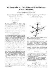
such a wave travelling at position x ′ along an axis that cuts the
Cartesian x-axis at an angle θ. In the continuous space-time domain,
solutions of this kind can be written
p(x ′ , t) = p 0 e st e −jkx′ , (9)
where p 0 is a real-valued amplitude value, s = σ + jω denotes
complex frequency, and k is the wavenumber. Using the coordinate
rotation x ′ = x cos(θ) + y sin(θ), this becomes
p(x, y, t) = p 0 e st e −jkxx e −jkyy , (10)
where k x = k cos θ and k y = k sin θ. In the discrete space-time
domain, the single-frequency plane-wave solution is:
p n l,m = p 0 e snT e −jˆk x lX e −jˆk y mX , (11)
where ˆk x and ˆk y denote the effective numerical wavenumbers,
which differ from the continuous-domain wavenumbers and are
related to a wavenumber ˆk associated with the propagation direction
along the x ′ -axis by
ˆk 2 = ˆk 2 x + ˆk 2 x. (12)
For solutions of this form, the approximation in (3) can be written
δ 2 t p n l,m = `z − 2 + z −1´ p n l,m,
= −4 sin 2 (ωT/2) p n l,m, (13)
where z = e sT , which represents the classic relationship between
the s- and the z-domain found in DSP literature. Hence by the
z-transform shift theorem, we have
p n+1
l,m = z p n l,m, (14)
which is easily veried by substituting both sides of Eq. (14) with
the form of Eq. (11). Similarly, under the assumption of singlefrequency
plane-wave solutions the spatial approximations in (4)
and (5) can be written
δxp 2 n l,m = −4 sin 2 (ˆk xX/2) p n l,m, (15)
δyp 2 n l,m = −4 sin 2 (ˆk y X/2) p n l,m. (16)
2.3. Von Neuman Stability Analysis
Classic von Neumann stability analysis investigates an FDTD scheme
for solutions of the form of Eq. (11), and seeks to establish a bound
on λ such that no growing solutions exist [1, 2]. From (14) it is
clear that any scheme is unstable for |z| > 1, hence the necessary
stability condition can be expressed as |z| ≤ 1. By substituting
(13), (15), and (16) into (6), the following equation in z can be
obtained:
z + 2B(s x , s y ) + z −1 = 0, (17)
where following [5] we introduce the new variables
s x = sin 2 (ˆk xX/2), (18)
s y = sin 2 (ˆk y X/2), (19)
and where
B(s x, s y) = 2λ 2 F (s x, s y) − 1, (20)
with
F (s x , s y ) =
s x + s y − 4bs xs y
1 − 4a(s x + s y ) + 16a 2 s x s y
. (21)
In FDTD literature, Eq. (17) is known as the amplication equation
or the amplication polynomial. The moduli of its two solutions
have to be smaller than or equal to unity for any combination
(s x , s y ) and thus any combination (ˆk x , ˆk y ). Since s x and
s y are periodic with π, it is sufcient to consider only real-valued
wavenumbers in the range −π/X ≤ ˆk x , ˆk y ≤ π/X. We note
that ˆk x and ˆk y can also become complex-valued [13], but in that
case only the real part has to be taken into account with regard to
stability analysis. From (17), it can be shown that |z| ≤ 1 when
B 2 (s x, s y) ≤ 1 (22)
which yields the bound on λ:
λ 2 ≤
1
F max (s x , s y )
(23)
For any (a, b) the function F (s x , s y ) reaches its maximum at one
of its extrema, where s x, s y ∈ [0, 1], thus
F max = max
„ «
1
1 − 4a , 2 − 4b
1 − 8a + 16a 2
1 − 8a + 16a2
2 − 4b
(24)
Therefore the necessary stability condition for the scheme in (6) is
«
λ 2 ≤ min
„1 − 4a, . (25)
Since λ 2 must be positive, it follows from (25) that we have the
auxiliary constraints:
a ≤ 1 4 , b ≤ 1 2 . (26)
DAFX-2