On the numerical solution of the 2D wave equation

More documents

Recommendations

Info

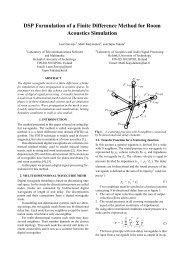
Proc. of the 11 th Int. Conference on Digital Audio Effects (DAFx-08), Espoo, Finland, September 1-4, 2008 SLF 90 o 135 o 45 o −180 o 0 o −135 o −45 o −90 o −180 o RLF 90 o 135 o 45 o −135 o −90 o −45 o 0 o INT(1/4) 135 o −180 o 90 o 45 o −135 o −90 o −45 o 0 o INT(1/6) [λ 2 = 0.75] 90 o INT(1/6) [λ 2 = 0.5] 90 o MFI 90 o 135 o 45 o 135 o 45 o 135 o 45 o −180 o −135 o −90 o −45 o 0 o −180 o −135 o −90 o −45 o 0 o −180 o −135 o −90 o −45 o 0 o FOA 90 o OPT 90 o 135 o 45 o 135 o 45 o color bar −180 o −135 o −90 o −45 o 0 o −180 o −135 o −90 o −45 o 0 o 0.7 0.8 0.9 1 relative phase velocity 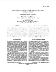Figure 3: Relative phase velocity as a function of frequency (polar plot radius) and propagation angle (polar plot angle). In each plot, starting from the most inner circle, the dotted-line circles indicate f = ( 1 8 , 1 4 , 3 8 , 1 2 )fs. comparing the schemes in that sense, let's specify this as the computational density required such that the deviation of the relative phase velocity from its ideal unity value is not larger than a critical error e c up to a critical frequency ω c. As a rst indication, we may dene the computational density simply as the number of nodal updates per square meter per second. This enables direct comparison between schemes that use exactly the same nodal update computations, such as all implicit schemes. Using this denition of computational density, we can dene the and although we have not explictly addressed alternative metrics, some tentative conclusions regarding implicit schemes could also be made for the separate case of membrane synthesis on basis of the analysis presented. following metric of relative efciency: ε(a, b, e c ) = ρnu(0, 0, ec, ωc) ρ nu (a, b, e c , ω c ) , (46) where ρ nu(a, b, e c, ω c) denotes the computational density for scheme (a, b) that meets the criterion (e c, ω c) and ρ nu(0, 0, e c, ω c) is the reference (SLF) scheme that we normalise by. Note that while ρ nu depends on the critical frequency, ε does not. The value of ρ nu is calculated by rst determining the sampling frequency required to meet the accuracy criterion, for which Eqs. (33) and (37) can be used. This involves rst determining the (normalised) frequencies ω a T and ω d T at which |1 − v a | and |1 − v d | are equal to e c . Because (33) and (37) are not directly invertable, this has to be done using optimisation methods. Once these critical frequencies have been found, the required sample rate DAFX-6
Proc. of the 11 th Int. Conference on Digital Audio Effects (DAFx-08), Espoo, Finland, September 1-4, 2008 relative phase velocity relative phase velocity 1.05 1 0.95 0.9 0.85 0.8 0.75 SLF RLF INT(1/4) INT(1/6) MFI FOA OPT AXIAL DIRECTIONS 0.7 0 0.1 0.2 0.3 0.4 0.5 normalised frequency 1.05 1 0.95 0.9 0.85 0.8 0.75 SLF RLF INT(1/4) INT(1/6) MFI FOA OPT DIAGONAL DIRECTIONS 0.7 0 0.1 0.2 0.3 0.4 0.5 normalised frequency Figure 4: Relative phase veloctiy for axial directions (top), and diagonal directions (bottom). ω is calculated as f s = c min(ω a T,ω d T ). The required spatial step X is then obtained directly from λ = (cT )/X. The required nodal density is thus ρ n = X −2 nodes per m 2 , and the required computational density (as in the number of nodal updates per m 2 per second) is ρ nu = Calculations of ε(a, b, e c ) have been performed for a large set (a, b) and a range of e c values. An example result (e c = 1%) is plotted in Fig. 5. fs . (X) 2 Table 2: Relative Efciency ε(e c ). scheme ε(10%) ε(1%) ε(0.1%) ε(0.01%) SLF 1.00 1.00 1.00 1.00 RLF 0.50 0.50 0.50 0.50 INT(1/4) 4.00 4.00 4.00 4.00 INT(1/6) 2.16 3.23 3.44 3.46 MFI 2.08 1.65 1.59 1.58 FOA 2.42 12.3 71.4 408 OPT 3.50 41.9 5.10 4.91 Table 2 shows the relative efciency of the special cases at their top Courant number for e c = 10%, 1%, 0.1%, and 0.01%. Note that one cannot directly compare values of different columns. Direct comparison is also not possible between schemes that use different amounts of nodes in their stencil, since this is not taken into account in the calculations. However, some important conclusions regarding such comparisons can still be drawn without getting into the messy business of counting FLOPS: • A nodal update with an interpolated scheme requires only a 0.25 0.2 0.15 0.1 0.05 0 −0.05 −0.1 −0.15 −0.2 −0.25 0 0.1 0.2 0.3 0.4 0.5 b Figure 5: Relative efciency (plotted as log 2 [ε(a, b, e c )]) for e c = 0.01. The optimal scheme lies in the white area. For any combination of the free parameters (a, b), the Courant number was chosen at the stability bound. a fraction of additional arithmetics in comparison with the SLF or the RLF scheme [10]. Hence it follows that the INT(1/4) is nearly 4 times more efcient than the SLF for any possible value of e c . • Inspection of results along the line a = 0 reveals the remarkable notion that amongst the explicit schemes, the INT(1/4) is always the optimally efcient scheme, regardless of the choice of e c . • Regarding implicit schemes (which all require exactly the same computational costs per nodal update for a given ADI implementation), the FOA scheme is the most efcient option, except when the cricital error is high, in which case a signicant better scheme can be found via optimisation. • As for comparing explicit schemes with implicit schemes, the computational costs of the ADI method per nodal update is roughly twice as much as that of explicit schemes [10]. Therefore it can be concluded that an implicit scheme that is more efcient than any explicit scheme can almost always be found, except if the critical error is chosen very high (e c > 2%). Additional insight can be gained by marking the positions of the various schemes on a map of the (a, b) domain (see Fig. 6). The solid line indicates the positions of optimised schemes when varying the critical error from e c = 10% to e c = 0.01%. The FOA scheme can be seen as the optimal scheme for e c → 0, and has the `maximally at' phase velocity error. Another interesting point is that the FOA scheme with λ at its top value uses a = − 1 + 1 4 2 √ , 3 thus is the `mirror-image' of the MFI scheme in the (a, b) domain. 4. CONCLUSIONS Compact FDTD schemes describe a useful group of nite difference methods and related techniques for simulation of acoustic systems governed by the wave equation. While considerable 5 0 −5 −10 −15 DAFX-7
Page 1 and 2: Proc. of the 11 th Int. Conference
Page 3 and 4: Proc. of the 11 th Int. Conference
Page 5: Proc. of the 11 th Int. Conference

On the numerical solution of the 2D wave equation

Create successful ePaper yourself

Delete template?

Save as template?