On the numerical solution of the 2D wave equation

Proc. of the 11 th Int. Conference on Digital Audio Effects (DAFx-08), Espoo, Finland, September 1-4, 2008
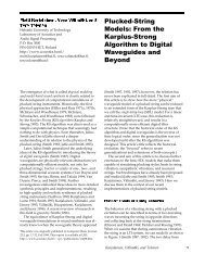
Stanfard Leap Frog (SLF) Rotated Leap Frog (RLF) Interpolated (INT) Implicit
(n+1)
(n)
(l-1,m-1) (l,m-1)
(l+1,m-1)
(l+1,m+1 )
(l+1,m)
(l-1,m-1) (l,m-1) (l+1,m-1)
(l+1,m)
(l+1,m+1 )
(l-1,m-1) (l,m-1) (l+1,m-1)
(l+1,m)
(l+1,m+1 )
(l-1,m-1) (l,m-1) (l+1,m-1)
(l+1,m)
(l+1,m+1 )
(n-1)
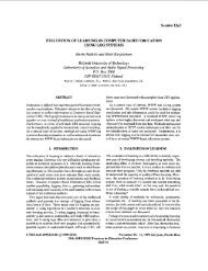
Figure 1: Compact FDTD Stencils. For each type of stencil, the middle node at time (n + 1) is updated using the remaining black-coloured
nodes.
3. ANALYSIS OF SPECIAL CASES
Table 1 lists seven special cases of compact schemes. The standard
leapfrog (SLF) scheme is mathematically equivalent to the rectilinear
digital waveguide mesh [8], and has exactly the same dispersion
relation as Yee's classic FDTD scheme [15, 2]. As explained
in [5], the rotated leap fog (RLF) scheme can be interpreted as applying
standard centered nite operators along the diagonals rather
than the horizontal and vertical axes. One could say that the RLF
stencil is 45 o rotated in comparison to the SLF scheme; both use
a “6-point stencil” in the space-time grid to update the new value
at time (n + 1) (see Fig. 1). Linear combinations of the SLF and
the RLF also exist, which result in a 10-point update stencil (see
Fig. 1). Such schemes, for which a = 0 and 0 < b < 1 2, have
been referred to as `interpolated schemes' [5]. We have listed two
special cases of interpolated schemes in Table 1. As a reference to
other studies, it is useful to point out that the interpolated scheme
with b = 1 and λ = p 1
6 2
is nearly equivalent to the interpolated
digital waveguide mesh [10], the latter having b = 0.1879.
Table 1: Special cases of compact FDTD schemes.
scheme a b stability bound
SLF 0 0 λ ≤ p 1
2
RLF 0
1
2
λ ≤ 1
INT(1/4) 0
1
4
λ ≤ 1
INT(1/6) 0
1
6
λ ≤ p 3
4
MFI
1
4 − 1
2 √ 3
FOA
1−λ 2
12
1
6
λ ≤ 1
1
λ ≤ √ 3 − 1
6
OPT 0.0492 0.228 λ ≤ 0.77
The remaining special cases in Table 1 are implicit schemes,
which use a 26-point update stencil (see Fig. 1). The maximally
at isotropic (MFI) scheme is the scheme for which the difference
between axial and diagonal relative phase velocity is maximally
at. Such a scheme is particularly useful when the aim is to apply
(off-line) pre- and post-warping techniques in order to remove as
much as possible any direction-independent numerical dispersion,
such as those presented in [9].
The implicit scheme with a = 1−λ2 and b = 1 12 6, originally
identied in [16], denes a subgroup of schemes within the familiy
of Eq. (6) of fourth-order accuracy (FOA), as can be seen directly
from Eq. (45).
The OPT scheme is an optimisation example, that is computationally
most efcient under the criterion that the relative phase
velocity error should not exceed 1% within any specied bandwidth
(see Sec. 3.2).
3.1. Relative Phase Velocity
In Fig. 2, the relative phase velocity, as calculated with (30), is
plotted as a function of the wavenumbers. What can be immediately
observed from these plots is how `isotropic' a particular
scheme is. For example, the INT(1/6) scheme (results plotted for
both λ 2 = 0.75, which is the stability bound, and λ 2 = 0.5,
which coincides with the interpolated digital waveguide mesh) and
the MFI scheme are far more `round' than the other special cases.
Note that the MFI scheme is the most isotropic of the three.
What is difcult - if not impossible - to determine from these
plots is the numerical dispersion at a certain frequency. In some
studies [11, 17], a circle is drawn on plots of this type with the intention
of indicating the “highest normalised temporal frequency”.
Unfortunately this does not work, since the wavenumbers (spatial
frequencies) are not proportional to the temporal frequencies (this
follows straight from the dispersion relation).
It is however possible to convert a set of wavenumbers (ˆk x, ˆk y)
to frequency ω (using Eq. (29)) and angle of propagation θ. This
way `polar plots' of the relative phase velocity can be generated,
where the polar radius corresponds to (normalised) frequency and
the polar angle indicates the direction (see Fig. 3). Now we may
draw circles on the plot in order to indicate particular frequencies.
These plots also immediately reveal the cut-off frequency
for any direction (beyond which waves in the discrete system are
evanescent and dispersion is of highly reduced relevance). As can
be seen, only the INT(1/4) scheme lls the complete bandwidth
up to Nyquist for all directions, while the SLF, the RLF, and the
INT(1/6) with λ 2 = 0.5 have the most `severe' cut-off frequencies
İt can also be observed from Fig. 3 that the FOA and the OPT
scheme have the largest bandwidth in which the numerical dispersion
remains relatively small. Amongst the explicit schemes, the
INT(1/6) (with λ 2 = 0.75) and the INT(1/4) scheme perform relatively
well in that regard.
A general observation that can be made is that the highest numerical
dispersion consistently occurs in either the axial or the diagonal
direction. Hence perhaps the most useful and informative
is to plot the relative phase velocity only for these directions, as
depicted in Fig. 4. This allows better to observe the exact value of
DAFX-4