Improving Gabor Noise - Sophia Antipolis - Inria

SUBMITTED TO IEEE TRANSACTIONS ON VISUALIZATION & COMPUTER GRAPHICS 1
Improving Gabor Noise
Ares Lagae, Sylvain Lefebvre, and Philip Dutré
Abstract— We have recently proposed a new procedural noise
function, Gabor noise, which offers a combination of properties
not found in existing noise functions. In this paper, we present
three significant improvements to Gabor noise: (1) an isotropic
kernel for Gabor noise, which speeds up isotropic Gabor noise
with a factor of roughly two, (2) an error analysis of Gabor noise,
which relates the kernel truncation radius to the relative error of
the noise, and (3) spatially varying Gabor noise, which enables
spatial variation of all noise parameters. These improvements
make Gabor noise an even more attractive alternative for existing
noise functions.
Index Terms— procedural noise, sparse convolution noise, Gabor
noise, isotropic Gabor kernel, circular Gabor filter, Hankel
transform, circularly symmetric functions, Gabor noise error
analysis, spatially varying Gabor noise
I. INTRODUCTION
Since its introduction by Perlin in 1985, procedural noise has
become an essential component in computer graphics [Ebert et al.,
2002]. Several noise functions have been proposed, for example
Perlin noise [Perlin, 2002], sparse convolution noise [Lewis,
1989], wavelet noise [Cook and DeRose, 2005] and anisotropic
noise [Goldberg et al., 2008]. For a recent survey of procedural
noise functions we refer the reader to Lagae et al..
We have recently proposed a new procedural noise function,
sparse Gabor convolution noise, or, in short, Gabor noise [Lagae
et al., 2009a] (section II). Gabor noise has several interesting
properties: it is procedural, it offers significant spectral control,
it supports anisotropy, it can be mapped onto surfaces without
using a parametrization, it can be filtered, and it is interactive. This
combination of properties is not found in existing noise functions.
In this paper, we present three significant improvements to
Gabor noise. As a first improvement, we present an isotropic
kernel for Gabor noise (section III). This improvement speeds
up isotropic Gabor noise with a factor of roughly two. This
can result in significant savings of 3D rendering time. Indeed,
in the 1990’s it was informally observed that “90% of 3D
rendering time is spent in shading, and 90% of that time is spent
computing Perlin noise” 1 . To our knowledge, the n-dimensional
real and even isotropic or circularly symmetric Gabor kernel
we derive is not known in literature. Zhang et al. [2002] have
presented a circular Gabor filter in the context of rotation-invariant
texture segmentation, but their filter is complex (that is, it has
an imaginary part), and is therefore not usable in the context
of Gabor noise. As a second improvement, we present an error
analysis of Gabor noise (section IV). This improvement relates
the kernel truncation radius, an important quality parameter of
Gabor noise, to the relative error of the noise, and replaces the
Ares Lagae is with the Katholieke Universiteit Leuven and REVES/INRIA
Sophia-Antipolis.
Sylvain Lefebvre is with REVES/INRIA Sophia-Antipolis and AL-
ICE/INRIA Nancy.
Philip Dutré is with the Katholieke Universiteit Leuven.
1 industry lore, as relayed by J.P. Lewis
ad hoc method to choose this parameter with a more principled
one. As a third improvement, we present spatially varying Gabor
noise (section V). This improvement enables spatial variation of
all noise parameters, a property not found in existing procedural
noise functions. This allows an artist to create spatially varying
procedural textures. Indeed, spatial variation of noise parameters
was shown to be useful in the context of non-procedural methods
related to Gabor noise [van Wijk, 1991, Ware and Knight, 1995,
Holten et al., 2006].
These three orthogonal improvements build upon and augment
the strong theoretical foundation of Gabor noise, and make
Gabor noise an even more attractive alternative for existing
noise functions. Although this paper focuses on procedural noise
for computer graphics, the family of methods that Gabor noise
belongs to is also relevant to visualization [van Wijk, 1991].
II. GABOR NOISE
In this section, we briefly review Gabor noise [Lagae et al.,
2009a]. We focus on its procedural nature and spectral control,
the two properties most relevant to this paper. Since this paper
addresses improvements to Gabor noise, we assume the reader is
generally familiar with Gabor noise.
Anisotropic Gabor noise is a sum of randomly weighted and
positioned Gabor kernels,
n K,F0 ,a,ω 0
(x, y) = X i
w i g K,F0 ,a,ω 0
(x − x i, y − y i), (1)
where the magnitude K, the frequency F 0 , the bandwidth a and
the orientation ω 0 are the noise parameters, g is the Gabor kernel,
{w i } are the random weights, and {(x i , y i )} are the random
positions. The Gabor kernel is the product of a radially symmetric
Gaussian and a 2D cosine,
g K,F0 ,a,ω 0
(x, y) =
K exp[−πa 2 (x 2 + y 2 )] cos[2πF 0(xcos ω 0 + y sin ω 0)], (2)
where K and a control the magnitude and width of the Gaussian,
and (F 0 , ω 0 ) is the frequency of the cosine. Anisotropic Gabor
noise is the convolution of sparse white noise and the Gabor
kernel,
" X
n K,F0 ,a,ω 0
(x, y) = w iδ (xi ,y i ) ∗ g K,F0 ,a,ω 0
#(x, y), (3)
i
where the random weights {w i } are distributed according to a
random variable W with a uniform distribution on the interval
[−1, +1], and the random positions {(x i , y i )} are distributed
according to a Poisson distribution with impulse density λ.
Because sparse white noise has a constant power spectrum, the
power spectrum of anisotropic Gabor noise is a scaled version of
the power spectrum of the Gabor kernel. The Gabor kernel in the
frequency domain is a pair of Gaussians,
G K,F0 ,a,ω 0
(f x, f y) =
K
n
2a exp − π ˆ(fx 2˜o
± F 2 a 2 0 cos ω 0) 2 + (f y ± F 0 sin ω 0) , (4)

SUBMITTED TO IEEE TRANSACTIONS ON VISUALIZATION & COMPUTER GRAPHICS 2
where K and a control the magnitude and width of the Gaussians,
and (F 0 , ω 0 ) and its symmetrical counterpart are the locations of
the Gaussians. Because the power spectrum of anisotropic Gabor
noise is a scaled version of the power spectrum of the Gabor
kernel, the parameters K, F 0 , a and ω 0 directly control the power
spectrum of the noise.
Isotropic Gabor noise is a sum of randomly weighted, positioned
and oriented Gabor kernels,
n K,F0 ,a(x, y) = X i
w i g K,F0 ,a(ω 0i , x − x i, y − y i), (5)
where the magnitude K, the frequency F 0 and the bandwidth
a are the noise parameters, and the random orientations {ω 0i }
are distributed according to a random variable Ω with a uniform
distribution on the interval [0, 2π). Similar to anisotropic Gabor
noise, the parameters K, F 0 and a directly control the power
spectrum of the noise.
The procedural evaluation of Gabor noise is similar to that of
Lewis’ [1989] sparse convolution noise and Worley’s [1996] cellular
texture basis function. Gabor noise is evaluated procedurally
by truncating the Gabor kernel and introducing a grid with a cell
size equal to the radius of the truncated kernel. This restricts
the evaluation of the noise to the grid cell containing the point
of evaluation and the eight neighboring grid cells. The Gabor
kernels in each cell are generated on-the-fly using a pseudorandom
number generator.
Next to its procedural nature and spectral control, Gabor noise
has several other interesting properties for computer graphics: it
supports anisotropy, it can be mapped onto surfaces without using
a parametrization, it can be filtered, and it is interactive. This is
the major difference between Gabor noise and related methods in
computer graphics, such as sparse convolution noise, and related
methods in visualization, such as spot noise [van Wijk, 1991,
Ware and Knight, 1995].
III. AN ISOTROPIC KERNEL FOR GABOR NOISE
Isotropic Gabor noise is defined using an anisotropic Gabor
kernel (see equation 5). In this section, we show that isotropic
Gabor noise can also be defined using an isotropic Gabor kernel,
and that the isotropic kernel has several advantages over the
anisotropic kernel. Most importantly, we show that isotropic
noise using the isotropic kernel is roughly two times faster than
isotropic noise using the anisotropic kernel.
We assume that the reader is familiar with circularly symmetric
functions (see appendix I), more specifically, with hyperspherical
coordinates (see appendix I-A), the integration (see appendix I-
B) and convolution (see appendix I-C) of circularly symmetric
functions, and the Hankel transform (see appendix I-D).
A. The Isotropic Gabor Kernel
We define the n-dimensional isotropic Gabor kernel similar
in spirit as other kinds of Gabor kernels: using a Gaussian and
a harmonic, which are related by multiplication in the spatial
domain, and by convolution in the frequency domain. We use
the Hankel transform (see appendix I-D), which is the method of
choice for working with Fourier transforms of isotropic or circularly
symmetric functions. We denote the n-dimensional isotropic
Gabor kernel, Gaussian, and harmonic as n I g (r), n I g G (r), and
n
I g H (r) in the spatial domain, and as n I G (fr), n I G G (f r), and
n
I G H (f r) in the frequency domain. We summarize their relations
as
spatial domain
frequency domain
n
I g G (r)
n
I g H (r)
n
I g (r) = n I g G (r) n I g H (r)
n H
⇐⇒
I G G (f r)
n H
n
,
⇐⇒
I G H (f r)
n H
⇐⇒ [ n I G G ∗ n I G H] (f r) = n I G(f r)
(6)
where n H
⇐⇒ denotes an order-n Hankel transform pair.
The Gaussian is a Gaussian in both the spatial domain and the
frequency domain. We define the Gaussian in the spatial domain,
n
I g G (r), as the circularly symmetric Gaussian,
n
I g G (r) = Ke −πa2 r 2 , (7)
where K and a are the magnitude and width of the Gaussian.
The Gaussian in the spatial domain is illustrated in figure 1(a) and
in figure 2(a). We obtain the Gaussian in the frequency domain,
n
I G G (f r), as the order-n Hankel transform of n I g G (r),
n
I G G (f r) = n H [ n I g G (r)]
= 2π Z ∞
Ke −πa2 r 2 J
f 1 2 n−1
1
2
n−1 (2πfrr) r 2 1 n dr
0
(8)
r
= K a n e− π a 2 f2 r
,
where J n is the order-n Bessel function of the first kind. The
Gaussian in the frequency domain is illustrated in figure 1(b) and
in figure 2(b).
The harmonic is typically defined as an impulse in the frequency
domain, located at the principal frequency, F 0 , of the
Gabor kernel. We therefore define the harmonic in the frequency
domain, n I G H (f r), as a circularly symmetric impulse,
n
I G H (f r) = δ (f r − F 0) , (9)
where F 0 is the frequency of the harmonic. The harmonic in the
frequency domain is illustrated in figure 1(d) and in figure 2(d).
We obtain the harmonic in the spatial domain, n I g H (r), as the
order-n Hankel transform of n I G H (f r),
n
I g H (r) = n H [ n I G H (f r)]
= 2π Z ∞
δ (f
r 1 r − F 0) J
2 n−1 1
2
n−1 (2πrfr) f 1 2 n
r df r
(10)
0
= 2π
r J 1 2 n−1 1 2 n−1 (2πF0r) F 2 1 n
0 .
The harmonic in the spatial domain is illustrated in figure 1(c)
and in figure 2(c).
We obtain the n-dimensional isotropic Gabor kernel in the
n
spatial domain, I g (r), as the multiplication of n I g G (r) and
n
I g H (r),
n
I g (r) = n I g G (r) n I g H (r)
= Ke −πa2 r 2 2πF 2 1 n
0
r J 1 2 n−1 2 1 n−1 (2πF0r) . (11)
The kernel in the spatial domain is illustrated in figure 1(e)
and in figure 2(e). We obtain the n-dimensional isotropic Gabor
kernel in the frequency domain, n I G(fr), as the convolution of
n
I G G (f r) and n I G H (f r). We simplify the convolution of isotropic
or circularly symmetric functions by exploiting their symmetry
(see appendix I-C). First, we convolve n I G G (f r) and n I G H (f r)
using this simplification,
n
I G (f r) = [ n I G G ∗ n I G H] (f r)
=
n−1
2π 2
Γ ` n−1
2
´
Z ∞
f ′ r =0 Z π
f φ =0
f ′ rn−1 sin n−2 f φ df ′ rdf φ ,
n
δ `f ′ r − F 0´ K
a n e− π a 2 (f 2 r +f ′ r 2 −2f rf ′ r cos f φ)
(12)

SUBMITTED TO IEEE TRANSACTIONS ON VISUALIZATION & COMPUTER GRAPHICS 3
Gaussian, Spatial Domain
Gaussian, Frequency Domain
K
I g G (r)
K/a
I G G (f r )
0
0 1/2a
r
0
0 a
f r
(a) Gaussian, spatial domain.
(b) Gaussian, frequency domain.
(a) Gaussian, spat. dom.
(b) Gaussian, freq. dom.
Harmonic, Spatial Domain
Harmonic, Frequency Domain
I 1 g H (r)
I 2 g H (r)
I 3 g H (r)
I 4 g H (r)
1
I G H (f r )
0
0 1/F 0
r
0
0 F 0
f r
(c) Harmonic, spatial domain.
(d) Harmonic, frequency domain.
(c) Harmonic, spat. dom.
(d) Harmonic, freq. dom.
Kernel, Spatial Domain
Kernel, Frequency Domain
I 1 g(r)
I 2 g(r)
I 3 g(r)
I 4 g(r)
I 1 G(f r )
I 2 G(f r )
I 3 G(f r )
I 4 G(f r )
0
0
r
0
0 F 0
f r
(e) Kernel, spatial domain.
(f) Kernel, frequency domain.
(e) Kernel, spat. dom.
(f) Kernel, freq. dom.
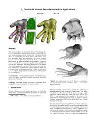
Fig. 1. The isotropic Gabor kernel. (a) Gaussian, spatial domain. (b)
Gaussian, frequency domain. (c) Harmonic, spatial domain. (d) Harmonic,
frequency domain. (e) Kernel, spatial domain. (f) Kernel, frequency domain.
Fig. 2. The 2D isotropic Gabor kernel. (a) Gaussian, spatial domain. (b)
Gaussian, frequency domain. (c) Harmonic, spatial domain. (d) Harmonic,
frequency domain. (e) Kernel, spatial domain. (f) Kernel, frequency domain.
where Γ is the Gamma function. Then, we integrate over f r.
′
Next, we simplify the convolution using the integral
Z π
„ «
sin n θ e x cos θ dθ = 2 n √
2 πx
− n 2
n + 1
I n
2
(x) Γ , (13)
2
0
where I n is the order-n modified Bessel function of the first
kind. Finally, we obtain
n
I G (f r) = 2πKF 1 2 n
„ «
0
e −π
a 2 2
f 1 n−1
a 2 (fr 2 +F2 0) 2πF0 I 12 n−1
a 2 fr . (14)
r
The kernel in the frequency domain is illustrated in figure 1(f)
and in figure 2(f).
B. Isotropic Gabor Noise using the Isotropic Gabor Kernel
We define n-dimensional isotropic Gabor noise using the
isotropic Gabor kernel similar to anisotropic (see equation 1) and
isotropic (see equation 5) Gabor noise using the anisotropic Gabor
kernel,
n
I n(x 1, . . . , x n) = X i
«
n
w i I g
„q(x 1 − x i,1) 2 + . . . + (x n − x i,n) 2
(15)
Note that, in contrast to the anisotropic kernel, the isotropic
kernel does not need to be randomly oriented. The variance of
the noise n I σ2 n is
n
I σn 2 = λE ˆW 2˜ Z ∞
S n
r=0
The power spectrum of the noise n I Snn is
n
I g 2 (r) r n−1 dr. (16)
n
I S nn (f r) = λE ˆW 2˜ | n I G(f r)| 2 . (17)
We provide equations for working with one-, two-, three- and
four-dimensional isotropic Gabor noise using the isotropic Gabor
kernel (see appendix II), including the isotropic Gabor kernel
in the spatial domain (see appendix II-A) and in the frequency
domain (see appendix II-B), the integral of the isotropic Gabor
kernel squared (see appendix II-C), the envelope of the isotropic
Gabor kernel (see appendix II-D), and the radius of the truncated
isotropic Gabor kernel (see appendix II-E).
C. Implementation, Results and Comparison
We have implemented isotropic Gabor noise using the isotropic
Gabor kernel, and we have verified most equations experimentally.
We evaluate the Bessel functions using code based on
Press et al. [2002, 6.5, 6.6] (polynomial approximations are also
available in Abramowitz and Stegun [1972, 9.4,9.8]), and the
Lambert-W function (see appendix II-E) using code based on
Keith [2009]. We verify the noise by comparing the estimated and
expected power spectrum and the actual and expected intensity
distribution [Lagae et al., 2009b].
.
We illustrate one-, two- and three-dimensional isotropic Gabor
noise using the isotropic Gabor kernel in figure 3, figure 4
and figure 5. Note the similarity between isotropic noise using
the isotropic kernel and isotropic noise using the anisotropic
kernel [Lagae et al., 2009a, figure 4]. Also note how closely
the estimated and expected power spectrum and the actual and
expected intensity distribution match.
We have found that isotropic noise using the isotropic kernel
is significantly faster than isotropic noise using the anisotropic
kernel. This is because of two reasons. First, the isotropic kernel

SUBMITTED TO IEEE TRANSACTIONS ON VISUALIZATION & COMPUTER GRAPHICS 4
Noise, Intensity Distribution
Noise, Intensity Distribution
4
3.5
actual intensity distribution
expected intensity distribution
90
80
actual intensity distribution
expected intensity distribution
3
70
normalized count / probability
2.5
2
1.5
normalized count / probability
60
50
40
30
1
20
0.5
10
0
-0.4 -0.3 -0.2 -0.1 0 0.1 0.2 0.3 0.4
0
-0.015 -0.01 -0.005 0 0.005 0.01 0.015
intensity
intensity
(a) Noise.
(b) Intensity distribution (histogram
and expected).
(a) Noise.
(b) Intensity distribution (histogram
and expected).
(c) Fourier transform (magnitude).
(d) Power spectrum estimate.
(e) Expected power spectrum.
(c) Fourier transform (magnitude).
(d) Power spectrum estimate.
(e) Expected power spectrum.
Noise, Power Spectrum
Noise, Power Spectrum
4.5
4
estimated power spectrum
expected power spectrum
1.2
estimated power spectrum
actual power spectrum
1
3.5
3
0.8
2.5
0.6
2
1.5
0.4
1
0.2
0.5
0
-1/2 -1/4 -1/8 0 1/8 1/4 1/2
f r
0
-1/2 -1/4 -1/8 0 1/8 1/4 1/2
f r
(f) Radial power spectrum (estimate
and expected).
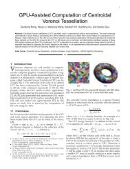
Fig. 4. 2D isotropic Gabor noise using the isotropic kernel. (a) Noise. (b)
Actual and expected intensity distribution. (c) Fourier transform (magnitude).
(d) Estimated power spectrum. (e) Expected power spectrum. (f) Estimated
and expected radial power spectrum.
(f) Radial power spectrum (estimate
and expected).
Fig. 5. 3D isotropic Gabor noise using the isotropic kernel. (a) Noise. (b)
Actual and expected intensity distribution. (c) Fourier transform (magnitude).
(d) Estimated power spectrum. (e) Expected power spectrum. (f) Estimated
and expected radial power spectrum.
Harmonic, Envelope
Kernel, Envelope
4
Noise, Spatial Domain
I 1 n(x)
0.35
Noise, Intensity Distribution
actual intensity distribution
expected intensity distribution
1
envelope of I gH (r)
2
envelope of I gH (r)
3
envelope of I gH (r)
4
envelope of I gH (r)
I 1 g E (r)
I 2 g E (r)
I 3 g E (r)
I 4 g E (r)
3
0.3
2
1
0
-1
-2
normalized count / probability
0.25
0.2
0.15
0.1
-3
0.05
0
0 1/F 0
0
0
-4
-100 -50 0 50 100
x
0
-4 -2 0 2 4
intensity
(a) Envelope of the harmonic.
r
(b) Envelope of the kernel.
r
(a) Noise.
(b) Intensity distribution (histogram
and expected).
Fig. 6. The envelope of the isotropic Gabor kernel. (a) Envelope of the
harmonic. (b) Envelope of the kernel.
9000
8000
7000
6000
5000
4000
3000
2000
1000
Noise, Frequency Domain
0
-1/2 -1/4 -1/8 0 1/8 1/4 1/2
f
| 1 N(x)| 2
(c) Fourier transform (magnitude).
9
8
7
6
5
4
3
2
1
Noise, Power Spectrum
0
-1/2 -1/4 -1/8 0 1/8 1/4 1/2
f
estimated power spectrum
expected power spectrum
(d) Power spectrum (estimate and expected).
Fig. 3. 1D isotropic Gabor noise using the isotropic kernel. (a) Noise. (b)
Actual and expected intensity distribution. (c) Fourier transform (magnitude).
(d) Estimated and expected power spectrum.
is more compact than the anisotropic kernel (see figure 1(e) and
figure 6). This results in a lower number of impulses per kernel for
the same impulse density, which in turn results in a shorter time
to evaluate the noise, since this time is directly proportional to the
number of impulses. Second, in contrast to the anisotropic kernel,
the isotropic kernel does not need to be randomly oriented (see
equation 5 and equation 15). This avoids the generation of random
orientations, which also results in a shorter time to evaluate the
noise. For example, for two-dimensional isotropic noise with
parameters K = 0.709645, a = 0.0443528 and F 0 = 0.0625,
where the kernel was truncated at 5% of its maximum value, the
radius of the kernel is 22.0169 for the anisotropic kernel, but only
15.6741 for the isotropic kernel, a reduction of 28.8086%, and for
an impulse density of λ = 0.0414605, the number of impulses per
kernel is 63.1386 for the anisotropic kernel, but only 32 for the

SUBMITTED TO IEEE TRANSACTIONS ON VISUALIZATION & COMPUTER GRAPHICS 5
(a) Perlin noise. (b) Wavelet noise. (c) Gabor noise,
anisotropic kernel.
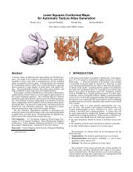
Fig. 7. A comparison of visual quality of different noise functions. (a)
Perlin noise. (b) Wavelet noise. (c) Gabor noise using the isotropic kernel.
Note that Perlin noise, and to a lesser degree also wavelet noise, both exhibit
an undesired axis-aligned anisotropy.
(a) Wavelet noise.
(b) Gabor noise, isotropic kernel.
Fig. 8. A comparison of filtering quality of different noise functions. (a)
Wavelet noise. (b) Gabor noise using the isotropic kernel. Each subfigure
shows a tilted plane with unfiltered noise on the left half and filtered noise on
the right half. Note that Gabor noise is better than wavelet noise at preserving
detail at high spatial frequencies in the far distance. Please also refer to
video 1.
on the parameter settings and the approximations used in the
implementation. With similar parameter settings as above, the
performance of Gabor noise is 144 FPS, and 255 FPS for half
the number of impulses per kernel. When approximating the
Poisson distribution by its mean, the performance is 198 FPS
and 357 FPS. The filtering quality of wavelet noise and Gabor
noise is illustrated in figure 8 and in video 1. We filter wavelet
noise by deriving a filtering weight by evaluating the filtering
Gaussian in the frequency domain at the principal frequency of the
noise. We filter Gabor noise by deriving new kernel parameters K,
F 0 and a by multiplying the filtering Gaussian in the frequency
domain with a Gaussian approximation of the isotropic kernel
in the frequency domain. In both cases, the anisotropic filtering
Gaussian in the frequency domain is approximated with an
isotropic one. Gabor noise enables a better filtering quality than
wavelet noise since Gabor noise is better than wavelet noise at
preserving detail at high spatial frequencies in the far distance.
This is clearly visible in video 1. This is because wavelet noise
only allows to apply a single filtering weight w to an entire noise
octave, while Gabor noise allows to adapt the frequency f and
bandwidth a of individual kernels. We have not included Perlin
noise in this comparison, since Cook and DeRose [2005, figure 1]
already showed that it is worse than wavelet noise in terms of
filtering quality, and because filtering Perlin noise in a principled
way is difficult since Perlin noise is not band-pass. We would
like to note that there are many other criteria that could also be
taken into account in a comparison [Lagae et al.], which might
or might not be relevant depending on the application.
Our results and comparison show that isotropic Gabor noise
using the isotropic Gabor kernel should be used whenever an
isotropic noise function is required with a higher quality than
Perlin noise and wavelet noise and a lower cost than isotropic
Gabor noise using the anisotropic Gabor kernel.
isotropic kernel, a reduction of 49.3179%. The time to evaluate
the noise using our CPU implementation is 4.11625 s for the
anisotropic kernel, but only 1.64481 s for the isotropic kernel, a
speedup of 2.50257 (512 × 512, Intel(R) Xeon(R) CPU 5160 at
3.00GHz). With similar parameter settings, the performance of
the noise using our GPU implementation is 77 FPS (frames per
second) for the anisotropic kernel, and 144 FPS for the isotropic
kernel, a speedup of 1.87 (512 × 512, NVIDIA Quadro FX 5800
GPU). We have found that the speedup is roughly independent of
the noise parameters. The speedup for three- and four-dimensional
isotropic noise should be even larger, since the isotropic kernel
gets more compact with increasing dimension (see figure 1(e) and
figure 6), and the number of random orientations that has to be
sampled gets larger with increasing dimension (see appendix I-A).
We have compared isotropic Gabor noise using the isotropic
kernel with Perlin noise [Perlin, 2002] and wavelet noise [Cook
and DeRose, 2005], two other isotropic noise functions. The
visual quality of these noise functions is illustrated in figure 7.
Perlin noise, and to a lesser degree also wavelet noise, both
exhibit an undesired axis-aligned anisotropy, which is not the
case for Gabor noise (also see [Lagae et al.]). We have measured
the performance of these noise functions using our GPU implementations.
The performance of Perlin noise is 3388 FPS, and
that of wavelet noise is 730 FPS (512 × 512, NVIDIA Quadro
FX 5800 GPU). The performance of Gabor noise is dependent
IV. AN ERROR ANALYSIS OF GABOR NOISE
The procedural evaluation of Gabor noise requires that the
Gabor kernel is truncated. This is typically done at a radius where
the envelope of the kernel reaches a sufficiently small value, for
example 5% of its maximum value [Lagae et al., 2009a, 4] [Lagae
et al., 2009b, 1]. However, this is an ad hoc approach, since
truncating the kernel introduces an error in the noise, and this
error is not quantified. In this section, we quantify the effect of
truncating the Gabor kernel, and we present a more principled
approach to truncate the Gabor kernel.
A. Relation of Kernel Truncation Radius to Noise Error
We relate the noise error resulting from truncating the Gabor
kernel g to the truncation radius r t . In this analysis, we use the
n-dimensional isotropic Gabor kernel (see section III), but the
analysis is also valid for other kernels, such as the anisotropic
Gabor kernel. We define a truncated Gabor kernel g t , where
j
g(r)
g t(r) =
0 ≤ rt < r
0 r t ≥ r
and an error kernel ∆g, where
j
0 0 ≤ rt < r
∆g(r) =
g(r) r t ≥ r
, (18)
. (19)
Note that g(r) = g t (r) + ∆g(r). We obtain the noise error ∆n
by subtracting the noise using the truncated kernel n t from the

SUBMITTED TO IEEE TRANSACTIONS ON VISUALIZATION & COMPUTER GRAPHICS 6
noise using the untruncated kernel n,
∆n (x 1, . . . , x n) = n(x 1, . . . , x n) − n t (x 1, . . . , x n)
= X i
w i∆g
“p
(x1 − x 1i ) 2 + . . . + (x n − x ni ) 2” .
(20)
Our key insight is that the noise error ∆n is, similar to Gabor
noise, a random pulse process [Lagae et al., 2009a, 2.2] [van
Etten, 2005, 8] [Papoulis and Pillai, 2002, 10.2]. The variance
σ∆n 2 of the noise error ∆n is therefore
σ∆n 2 = λ E ˆW 2˜ Z ∞
S n ∆g 2 (r)dr. (21)
We define the root mean square error and the relative error using
the variances σn 2 and σ∆n 2 of the noise and the noise error. We
define the root mean square error e RMS as the square root of the
variance of the noise error,
q
e RMS = σ∆n 2 . (22)
We define the relative error e as the root mean square error e RMS
over the root mean square amplitude p σn,
2
s R ∞
e = eRMS 0
√ = σ
2 n
∆g 2 (r) dr
R ∞
0
g 2 (r) dr = s1 −
0
R rt
0 g2 (r) dr
R ∞
0
g 2 (r) dr . (23)
6
4
2
0
-2
-4
-6
Error Analysis Isotropic 1D Noise
-100 -50 0 50 100
x
procedural implementation
reference implementation
error
root mean square error
expected root mean square error
(a) High relative error.
3
2
1
0
-1
-2
-3
Error Analysis Isotropic 1D Noise
-100 -50 0 50 100
x
procedural implementation
reference implementation
error
root mean square error
expected root mean square error
(b) Low relative error.
Fig. 9. An error analysis of 1D isotropic Gabor noise. (a) Noise with a high
relative error (e = 25%). (b) Noise with a low relative error (e = 1%). Each
subfigure shows a graph and three images. The graph shows the noise using
the untruncated kernel (n) (reference implementation), the noise using the
truncated kernel (n t) (procedural implementation), the noise error (∆n), the
actual root mean square noise error, and the estimated root mean square noise
error (e RMS ). The three images show the noise using the untruncated kernel
(n), the noise using the truncated kernel (n t), and the noise error (∆n).
Note that the relative error e only depends on the kernel g and
the truncation radius r t , and not on the parameters of the sparse
white noise λ and W . Our analysis allows to determine the relative
noise error for a given kernel truncation radius, but also allows to
determine the kernel truncation radius for a given relative error,
by solving equation 23 for r t . The usage of relative error in this
context is motivated by Weber’s Law [Blackwell, 1972]. This is
a much more principled approach than truncating the kernel at an
arbitrarily chosen value.
B. Implementation, Results and Discussion
We have implemented the noise error analysis and we have verified
the equations experimentally. For most kernels, a closed-form
expression for R ∞
0 g2 (r) dr is available (see appendix II-C), but
a closed-form expression for R r t
0 g2 (r) dr is not. Therefore, we
generally solve equation 23 for r t numerically, using bracketing
and bisection [Press et al., 2002, 9.1], the closed-form expression
to evaluate R ∞
0 g2 (r) dr, and Simpson’s rule [Press et al., 2002,
4.2] to evaluate R r t
0 g2 (r) dr. Note that for isotropic noise using
the isotropic kernel, all integrals are one-dimensional.
We illustrate the error analysis of one-dimensional isotropic
noise using the isotropic kernel in figure 9. Note how closely the
actual and expected root mean square error match. We illustrate
the error analysis of two-dimensional isotropic noise using the
isotropic kernel in figure 10. We plot the relative error versus the
kernel radius for one-, two-, three- and four-dimensional isotropic
noise using the isotropic kernel in figure 11. Note that the relative
error quickly decreases with increasing kernel truncation radius.
We now revisit the example of subsection III-C. When truncating
the kernel using a relative error of 2%, the radius of the
kernel is 25.25 for the anisotropic kernel, but only 20.8984 for the
isotropic kernel, a reduction of 17.2341%, the number of impulses
per kernel is 46.7139 for the anisotropic kernel, but only 32 for
the isotropic kernel, a reduction of 31.498%, and the time to
evaluate the noise using our CPU implementation is 2.50428 s
for the anisotropic kernel, but only 1.02537 s for the isotropic
kernel, a speedup of 2.44233. We generalize this example and
(a) High relative error.
(b) Low relative error.
Fig. 10. An error analysis of 2D isotropic Gabor noise. (a) Noise with
a high relative error (e = 25%). (b) Noise with a low relative error
(e = 1%). Each subfigure shows the noise using the untruncated kernel
(n) (reference implementation), the noise using the truncated kernel (n t)
(procedural implementation), and the noise error (∆n).
plot the relative error versus the kernel radius for two-dimensional
isotropic noise using the anisotropic and the isotropic kernel in
figure 12. This figure shows that for the same truncated kernel
radius, the relative error is always smaller for the isotropic kernel
than for the anisotropic kernel, and for the same relative error,
the isotropic kernel is always smaller and therefore faster than
the anisotropic kernel.
We believe that in general equation 23 should be used rather
than the ad hoc approach to determine the radius of the truncated
kernel, except for reasons of computational expense, for example
in the case of spatially varying noise (see section V), or simplicity.
V. SPATIALLY VARYING GABOR NOISE
The procedural evaluation of Gabor noise introduces a grid with
a cell size equal to the radius of the truncated kernel [Lagae et al.,
2009a, 4]. This restricts the evaluation of the noise to the grid cell

SUBMITTED TO IEEE TRANSACTIONS ON VISUALIZATION & COMPUTER GRAPHICS 7
Relative Error vs Kernel Radius
Kernel Radius vs Relative Error
25
isotropic 1D noise
isotropic 2D noise
isotropic 3D noise
isotropic 4D noise
50
isotropic 1D noise
isotropic 2D noise
isotropic 3D noise
isotropic 4D noise
20
45
relative error (%)
15
10
kernel radius
40
35
30
5
25
1
25 30 35 40 45 50
25
20
15
10
5
1
kernel radius
relative error (%)
(a) Relative error vs. kernel radius.
(b) Kernel radius vs. relative error.
Fig. 11. Relative error versus kernel radius for isotropic Gabor noise using
the isotropic kernel. (a) Relative error versus kernel radius. (b) Kernel radius
versus relative error.
(a) grids (b) α = 0 (c) α = 0.25
Relative Error vs Kernel Radius for Isotropic 2D Noise
Kernel Radius vs Relative Error
25
isotropic kernel
anisotropic kernel
50
isotropic kernel
anisotropic kernel
20
45
40
relative error (%)
15
10
kernel radius
35
30
(d) α = 0.50 (e) α = 0.75 (f) α = 1
5
1
25 30 35 40 45 50
kernel radius
(a) Relative error vs. kernel radius.
25
25
20
15
relative error (%)
(b) Kernel radius vs. relative error.
Fig. 12. Relative error versus kernel radius for 2D isotropic Gabor noise
using the anisotropic and the isotropic kernel (a) Relative error versus kernel
radius. (b) Kernel radius versus relative error.
10
5
1
Fig. 13. The hierarchy of grids used in spatially varying Gabor noise. (a) The
grids at level l 0 (red) and l 1 (blue). (b-f) The weighted combined impulses of
both grids for different kernel radii. Note that the red points disappear faster
than the blue points appear.
1
Weighting Functions
w 0
w 1
0.8
containing the point of evaluation and the eight neighboring grid
cells. However, this also prohibits spatial variation of the noise
parameters, since the kernel radius, and therefore the cell size,
is in general dependent on these parameters. In this section, we
present a procedural evaluation of Gabor noise that enables noise
with spatially varying parameters.
Fig. 14.
0.6
0.4
0.2
0
0 0.2 0.4 0.6 0.8 1
The weighting functions used in spatially varying Gabor noise.
A. Procedural Evaluation of Gabor Noise with Spatially Varying
Parameters
Evaluating Gabor noise using a single grid is optimal for a
single kernel radius corresponding to a fixed set of noise parameters.
In order to handle arbitrary kernel radii, corresponding to
arbitrary or noise parameters, we use a hierarchy of grids, where
the cell size of consecutive grids differs by a factor of two. More
specifically, the grid at level l of the hierarchy has a cell size of 2 l .
This implies that the grid at level l is optimal for a kernel radius
r l = 2 l . We have observed that, for different noise parameters, an
equal noise quality is obtained by maintaining a constant number
of impulses N per kernel area. Therefore, we associate the grid at
level l with an impulse density of λ l = N/πrl 2 . When evaluating
the noise using an arbitrary kernel radius r, we use the two grids
with kernel radii r 0 and r 1 that bracket r. These are the grids
with level l 0 = ⌊log 2 r⌋ and l 1 = l 0 + 1, for which r 0 ≤ r < r 1 .
We parametrize the radius r in terms of r 0 and r 1 by introducing
a parameter α in [0, 1) such that r = (1 − α)r 0 + αr 1 . When
evaluating the noise, we combine the impulses of both grids by
weighing the contribution due to each grid,
n(x, y) =w 0(α) X i 0
w i0 g(x − x i0 , y − y i0 )
+w 1(α) X i 1
w i1 g(x − x i1 , y − y i1 ),
(24)
where the first and second term correspond to the grid with
level l 0 and l 1 , and w 0 and w 1 are weighting functions. This
is illustrated in figure 13. It is important to note that this is a
linear combination of two noises with the same parameters, and
that the goal of the interpolation is to transition between grids
with different impulse densities, and not to obtain a noise with
interpolated parameters. Interpolating between two noises with
frequencies F 0 and F 1 (for example two octaves of Perlin noise)
cannot produce a noise with an intermediate frequency F , due to
the linearity of the Fourier transform, while interpolating between
two noises that already have frequency F obviously can.
For obvious reasons, we require that w 0 (0) = 1, that w 0 (1) =
0, and that w 0 is monotonically decreasing, and similarly that
w 1 (0) = 0, that w 1 (1) = 1, and that w 1 is monotonically
increasing. However, several choices for w 0 and w 1 remain. A
simple option is to choose w 0 (α) = 1−w(α) and w 1 (α) = w(α),
where w(α) is the linear weighting function w(α) = α or the
cubic weighting function w(α) = 3α 2 − 2α 3 . However, the
resulting weighting functions do not result in visually pleasing
transitions. This is illustrated in video 2. The weighting functions
can be determined by imposing additional constraints. For
example, imposing the constraint that the power spectrum of
both sides of equation 24 is the same leads to w 0 (α)(1 + α) +
w 1 (α)(1+α)/2 = 1. We have noticed that the visually unpleasing
transitions are caused by the fact that the two grids have a different
impulse density. The number of impulses per kernel area N 0
due to the grid with level l 0 equals N 0 = (1 + α) 2 N, while
the number of impulses per kernel area N 1 due to the grid with
level l 1 equals N 1 = N 0 /4. Therefore, we impose the constraint
that the weighted number of impulses per kernel area remains
constant, more specifically such that w 0 (α)N 0 + w 1 (α)N 1 = N
or equivalently such that w 0 (α)(1 + α) 2 + w 1 (α)(1 + α) 2 /4 = 1.
We now choose w 0 (α)(1+α) 2 = 1−w(α) and w 1 (α)(1+α) 2 /4 =

SUBMITTED TO IEEE TRANSACTIONS ON VISUALIZATION & COMPUTER GRAPHICS 8
Fig. 15. Spatially varying 2D Gabor noise. The noise parameters vary from K = 0.7096, F 0 = 0.03125 and a = 0.02218 at the left to K = 0.7096,
F 0 = 0.25 and a = 0.1774 at the right. The value of α is visualized at the bottom of the image. Note that this image spans four grid levels.
w(α), where w(α) is a weighting function. The simplest option
for w(α) is the linear weighting function w(α) = α, which also
satisfies the power spectrum constraint, and which results in the
weighting functions
w 0 (α) =
1 − α
(1 + α) 2 (25)
4α
w 1 (α) =
(1 + α) 2 . (26)
This is illustrated in figure 14. These weighting functions result
in visually pleasing transitions. This is illustrated in video 2.
B. Implementation, Results, Comparison and Discussion
We have implemented spatially varying Gabor noise and we
have verified the equations experimentally. Note that in contrast
with regular Gabor noise, the evaluation of spatially varying
Gabor noise includes the computation of the kernel truncation
radius. Because of computational expense, we use the ad hoc
approach (see section IV). Also note that the noise evaluation
is not restricted to exactly nine grid cells, and that the seeding
strategy has to take into account the grid level.
We illustrate spatially varying 2D Gabor noise in figure 15 and
video 2. We show procedural textures generated with spatially
varying surface Gabor noise in figure 16. Note that the simple
alternative of warping the domain variables of a regular Gabor
noise to obtain spatially varying Gabor noise might work in the
case of a 2D noise, as in figure 15, but would probably not work
in the case of spatially varying surface noise, as in figure 16, and
might be problematic for filtering.
We have compared the performance of spatially varying Gabor
noise and regular Gabor noise. The hierarchical solution of
spatially varying Gabor noise is only roughly a factor two slower
than regular Gabor noise. We have also compared the performance
of Perlin noise, regular Gabor noise and spatially varying Gabor
noise in the specific case of figure 16. The performance of Perlin
noise was 763 FPS, that of regular Gabor noise 22.8 FPS, and that
of spatially varying Gabor noise 20.6 FPS (2 octaves, 1024×1024,
NVIDIA Quadro FX 3800 GPU). In this specific case, spatially
varying Gabor noise is almost as fast as regular Gabor noise.
Perlin noise is significantly faster than Gabor noise, but also lacks
several attractive features of Gabor noise such as spatial variation
and filtering.
A somewhat similar mechanism as the one used for spatially
varying Gabor noise was recently used by Benard et al. [2010]
to construct a dynamic noise primitive for coherent stylization in
expressive rendering.
VI. CONCLUSION
In this paper, we have presented three significant improvements
to Gabor noise: an isotropic kernel for Gabor noise, which speeds
up isotropic Gabor noise with a factor of roughly two, an error
analysis of Gabor noise, which relates the kernel truncation radius
to the relative error of the noise, and spatially varying Gabor
noise, which enables spatial variation of all parameters. These
improvements build upon and augment the strong theoretical
foundation of Gabor noise, and make Gabor noise an even more
attractive alternative for existing noise functions.
ACKNOWLEDGMENT
We would like to thank the anonymous reviewers. We are grateful
to the NVIDIA Professor Partnership Program for equipment
donations. Ares Lagae is a Postdoctoral Fellow of the Research
Foundation - Flanders (FWO), and acknowledges K.U.Leuven
CREA funding (CREA/08/017). Sylvain Lefebvre receives support
from the Agence Nationale de la Recherche (SIMILAR-
CITIES ANR-2008-COORD-021).
REFERENCES
Milton Abramowitz and Irene A. Stegun. Handbook of Mathematical
Functions with Formulas, Graphs and Mathematical
Tables. Dover, 1972. Ninth Dover printing, with corrections.
Pierre Benard, Ares Lagae, Peter Vangorp, Sylvain Lefebvre,
George Drettakis, and Joelle Thollot. A dynamic noise primitive
for coherent stylization. Computer Graphics Forum (Proceedings
of the 20th Eurographics Symposium on Rendering),
29(4):1497–1506, 2010.
H. R. Blackwell. Luminance difference thresholds. In D. Jameson
and L. M. Hurvich, editors, Handbook of Sensory Physiology,
volume VII/4, pages 86–99. Springer-Verlag, Berlin, 1972.
Ronald N. Bracewell. The Fourier Transform and its Applications.
McGraw-Hill, 3rd edition, 2000. International editions 2000.
Ronald N. Bracewell. Fourier Analysis and Imaging. Springer,
2004.
Robert L. Cook and Tony DeRose. Wavelet noise. ACM
Transactions on Graphics, 24(3):803–811, 2005.
David S. Ebert, F. Kenton Musgrave, Darwyn Peachey, Ken Perlin,
and Steven Worley. Texturing and Modeling: A Procedural
Approach. Morgan Kaufmann Publishers, Inc., 3rd edition,
2002.
A. Goldberg, M. Zwicker, and F. Durand. Anisotropic noise. ACM
Transactions on Graphics, 27(3):54:1–54:8, 2008.
Danny Holten, Jarke J. Wijk, Van, and Jean-Bernard Martens. A
perceptually based spectral model for isotropic textures. ACM
Transactions on Applied Perception, 3(4):376–398, 2006.

SUBMITTED TO IEEE TRANSACTIONS ON VISUALIZATION & COMPUTER GRAPHICS 9
Briggs Keith. Lambert W function. http://keithbriggs.
info/software/LambertW.c, 2009.
A. Lagae, S. Lefebvre, R. Cook, T. DeRose, G. Drettakis, D. S.
Ebert, J. P. Lewis, K. Perlin, and M. Zwicker. A survey of
procedural noise functions. Computer Graphics Forum. to
appear.
Ares Lagae, Sylvain Lefebvre, George Drettakis, and Philip
Dutré. Procedural noise using sparse Gabor convolution. ACM
Transactions on Graphics, 28(3):54:1–54:10, 2009a.
Ares Lagae, Sylvain Lefebvre, George Drettakis, and Philip Dutré.
Procedural noise using sparse Gabor convolution - auxiliary
material. Report CW 545, Department of Computer Science,
K.U.Leuven, Celestijnenlaan 200A, 3001 Heverlee, Belgium,
May 2009b.
J. P. Lewis. Algorithms for solid noise synthesis. In Computer
Graphics (Proceedings of ACM SIGGRAPH 89), volume 23,
pages 263–270, 1989.
Athanasios Papoulis and Unnikrishna Pillai. Probability, Random
Variables and Stochastic Processes. McGraw-Hill, 4rd edition,
2002.
Ken Perlin. Improving noise. In Proceedings of ACM SIGGRAPH
2002, pages 681–682, 2002.
William H. Press, William T. Vetterling, Saul A. Teukolsky, and
Brian P. Flannery. Numerical Recipes in C++. Cambridge
University Press, 2nd edition, 2002.
Wim C. van Etten. Introduction to Random Signals and Noise.
Wiley, 2005.
Jarke J. van Wijk. Spot noise texture synthesis for data visualization.
In Computer Graphics (Proceedings of ACM SIGGRAPH
91), volume 25, pages 309–318, 1991.
Colin Ware and William Knight. Using visual texture for
information display. ACM Transactions on Graphics, 14(1):
3–20, 1995.
Steven Worley. A cellular texture basis function. In Proceedings
of ACM SIGGRAPH 1996, pages 291–294, 1996.
Jainguo Zhang, Tieniu Tan, and Li Ma. Invariant texture segmentation
via circular Gabor filters. In Proceedings of the 16th
International Conference on Pattern Recognition, volume 2,
pages 901–904 vol.2, 2002.
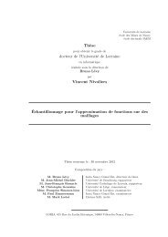
Fig. 16. Procedural textures generated with spatially varying surface Gabor
noise. (top) A rusty car. (bottom) A dragon covered in scales. The spatial
variation in the size of the rust patterns and the scales is steered by surface
curvature.
coordinates, φ 1 , . . . , φ n−1 , where
APPENDIX I
CIRCULARLY SYMMETRIC FUNCTIONS
In this section we cover circularly symmetric functions. We
review hyperspherical coordinates (subsection I-A) and the integration
of circularly symmetric functions (subsection I-B), we
simplify the convolution of circularly symmetric functions (subsection
I-C), and we review the Hankel transform (subsection I-
D).
x 1 = r cos φ 1
x 2 = r sin φ 1 cos φ 2
.
, (27)
x n−1 = r sin φ 1 . . . sin φ n−2 cos φ n−1
x n = r sin φ 1 . . . sin φ n−2 sin φ n−1
where r ∈ [0, ∞), φ 1 . . . φ n−2 ∈ [0, π) and φ n−1 ∈ [0, 2π). The
corresponding volume element is
r n−1 sin n−2 φ 1 sin n−3 φ 2 . . . sin φ n−2 dr dφ 1 . . . dφ n−1. (28)
A. Hyperspherical Coordinates
The hyperspherical coordinate system, the generalization of
two-dimensional polar coordinates and three-dimensional spherical
coordinates, is a natural coordinate system for working with
circularly symmetric functions. The hyperspherical coordinates
of a point in n-dimensional space with Cartesian coordinates
(x 1 , . . . , x n) consist of a radial coordinate, r, and n − 1 angular
B. Integration of Circularly Symmetric Functions
The integration of circularly symmetric functions can be simplified
by exploiting their symmetry. When a function f is circularly
symmetric in n dimensions, then the integral of f over R n reduces

SUBMITTED TO IEEE TRANSACTIONS ON VISUALIZATION & COMPUTER GRAPHICS 10
to a one-dimensional integral,
Z +∞
. . .
Z +∞
x 1 =−∞ x n=−∞
f (x 1, . . . , x n) dx 1 . . . dx n
Z ∞
= S n f (r) r n−1 dr, (29)
r=0
where S n is the hyper-surface area of an n-sphere of unit radius,
where J n is the order-n Bessel function of the first kind.
The Hankel transform is strictly reciprocal. An order-n Hankel
transform pair is denoted as f (r) n H
⇐⇒ F (f r). For n = 1, the
Hankel transform corresponds to the Fourier transform, since
circularly symmetric functions are real and even, and J 1/2 (x) =
(2/πx) 1/2 sin x and J −1/2 (x) = (2/πx) 1/2 cos x.
where Γ is the Gamma function.
S n = 2π n 2
´, (30)
Γ` n
2
C. Convolution of Circularly Symmetric Functions
We simplify the convolution of circularly symmetric functions
by exploiting their symmetry. First, we formulate the convolution
of two n-dimensional circularly symmetric functions f and g
using hyperspherical coordinates (see subsection I-A) as
[f ∗ g] (r) =
Z ∞
r ′ =0
Z π
φ ′ 1 =0 . . .
Z π
φ ′ n−2 =0 Z 2π
f `r ′´ g (R) r ′n−1
φ ′ n−1 =0
sin n−2 φ ′ 1 sin n−3 φ ′ 2 . . . sin φ ′ n−2
dr ′ dφ ′ 1 . . . dφ ′ n−1, (31)
where R 2 = r 2 +r ′2 −2rr ′ cos φ ′ 1. We set the angular coordinates
φ ′ 1 . . . φ ′ n−1 to zero in the expression for R 2 , since all functions
are circularly symmetric, leaving only the angular coordinate φ ′ 1.
Next, we simplify the convolution using the integral
Z π
sin n θ dθ = √ π Γ ` n+1
2
0
Γ ` ´, (32)
n+2
2
where Γ is the Gamma function. Finally, we obtain
[f ∗ g] (r) =
n−1
2π 2
´
Z ∞
Z π
Γ ` n−1
2 r ′ =0 φ=0
(33)
with R 2 = r 2 + r ′2 − 2rr ′ cos φ. For n = 2, equation 33
corresponds to the equation given in Bracewell [2000, table 13.3].
´
f `r ′´ g (R) r ′n−1 sin n−2 φ dr ′ dφ,
APPENDIX II
EQUATIONS FOR ISOTROPIC GABOR NOISE USING THE
ISOTROPIC GABOR KERNEL
In this section, we provide equations for working with one-
, two-, three- and four-dimensional isotropic Gabor noise using
the isotropic Gabor kernel. We provide equations for the isotropic
Gabor kernel in the spatial domain (subsection II-A) and in the
frequency domain (subsection II-B), the integral of the isotropic
Gabor kernel squared (subsection II-C), the envelope of the
isotropic Gabor kernel (subsection II-D), and the radius of the
truncated isotropic Gabor kernel (subsection II-E).
A. The Isotropic Gabor Kernel in the Spatial Domain
We obtain the one-, two-, three- and four-dimensional isotropic
Gabor kernel in the spatial domain from equation 11, keeping into
account that that J 1/2 (x) = (2/πx) 1/2 sin x and J −1/2 (x) =
(2/πx) 1/2 cos x. The one-, two-, three- and four-dimensional
isotropic Gabor kernel in the spatial domain is
1
Ig (r) = Ke −πa2 r 2 2cos (2πF 0r) , (35)
2
Ig (r) = Ke −πa2 r 2 2πF 0J 0 (2πF 0r) , (36)
3
Ig (r) = Ke −πa2 r 2 2F 0
sin (2πF0r) , (37)
r
4
Ig (r) = Ke −πa2 r 2 2πF0
2 J 1 (2πF 0r) . (38)
r
We illustrate the isotropic Gabor kernel in the spatial domain in
figure 1(e) and in figure 2(e).
D. The Hankel Transform
The Hankel transform [Bracewell, 2000, 13] [Bracewell, 2004,
9] is the method of choice for working with Fourier transforms
of circularly symmetric functions.
When a function f is circularly symmetric in n dimensions,
that is, when f (x 1 , . . . , x n) = f (r), where r 2 = x 2 1 + . . . +
x 2 n, then F , the n-dimensional Fourier transform of f, is also
circularly symmetric, that is, F (f x1 , . . . , f xn ) = F (f r), where
fr 2 = fx 2 1
+ . . . + fx 2 n
. The relation between the one-dimensional
functions f (r) and F (f r) is given by the Hankel transform of
order n. More specifically, the n-dimensional Fourier transform
of f (x 1 , . . . , x n) is given by the order-n Hankel transform
of f (r), that is,
n F [f (x 1 , . . . , x n)] = n H [f (r)]. Note that,
somewhat counterintuitively, the n-dimensional Fourier transform
of f (x 1 , . . . , x n) is not equal to the one-dimensional Fourier
transform of f (r), that is, n F [f (x 1 , . . . , x n)] ≠ 1 F [f (r)].
The Hankel transform, also called the Fourier-Bessel transform,
is a one-dimensional integral transform with a Bessel function
kernel. The Hankel transform of order n is
n H [f (r)] = F (f r) =
2π Z ∞
f (r) J 1
2
n−1 (2πfrr) r 1 2 n dr,
f 1 2 n−1
r
0
(34)
B. The Isotropic Gabor Kernel in the Frequency Domain
We obtain the one-, two-, three- and four-dimensional isotropic
Gabor kernel in the frequency domain from equation 14, keeping
into account that I 1/2 (x) = (2πx) −1/2 `e x − e −x´ and
I −1/2 (x) = (2πx) −1/2 `e x + e −x´. The one-, two-, three- and
four-dimensional isotropic Gabor kernel in the frequency domain
is
1
IG (f r) = K a
2
IG (f r) = 2πKF0
“e −π
a 2 (fr−F 0) 2 + e −π
a 2 (fr+F 0) 2” , (39)
a 2
e −π
a 2 (f 2 r +F2 0) I0
„ 2πF0
a 2 fr «
, (40)
“
3
IG (f r) = KF0 e −π
a
af 2 (fr−F 0) 2 − e −π
a 2 (fr+F 0) 2” , (41)
r
4
IG (f r) = 2πKF „ «
0
2 e −π
a 2 a
f 2 (fr 2 +F2 0) 2πF0
I1
r
a 2 fr . (42)
We illustrate the isotropic Gabor kernel in the frequency domain
in figure 1(f) and in figure 2(f).
C. The Integral of the Isotropic Gabor Kernel Squared
We obtain the integral of the isotropic Gabor kernel squared
by integrating the Gabor kernel squared in the spatial domain or

SUBMITTED TO IEEE TRANSACTIONS ON VISUALIZATION & COMPUTER GRAPHICS 11
in the frequency domain. The integral of the one-, two-, threeand
four-dimensional isotropic Gabor kernel squared is
Z ∞
√ „ «
1
2 Ig 2 2K
2
(r) dr = 1 + e − 2πF 0
a
r=0
a
2 (43)
Z ∞
„ «
2
2π Ig 2 (r) rdr = 2π2 K 2 F0
2 e − πF2 0 πF
2
r=0
a 2 a 2 I 0
0 (44)
a 2
Z ∞
3
4π Ig 2 (r) r 2 dr = 2√ „ «
2πK 2 F0
2 1 − e − 2πF 0
a
r=0
a
2 (45)
Z ∞
„ «
2π 2 4
Ig 2 (r) r 3 dr = 2π3 K 2 F0
4 e − πF2 0 πF
2
a 2 a 2 I 0
1 . (46)
a 2
r=0
Ares Lagae is a Postdoctoral Fellow of the Research
Foundation - Flanders (FWO), working at the Computer
Graphics Research Group of the K.U.Leuven.
He received the MS and BS degrees in computer
science from the K.U.Leuven in 2000 and 2002.
He received the PhD degree in computer science
from the K.U.Leuven in 2007, working with Philip
Dutré. He spent the academic year 2009 - 2010 at
REVES, INRIA Sophia Antipolis - Méditerranée,
working with George Drettakis. Since 2007, he is
a Postdoctoral Fellow of the Research Foundation
- Flanders (FWO). More details about his research can be found at http:
//people.cs.kuleuven.be/˜ares.lagae/.
D. The Envelope of the Isotropic Gabor Kernel
We define the envelope of the isotropic Gabor kernel as the
product of the Gaussian with the envelope of the harmonic. The
envelope of cos(x) and sin (x) is 1, and the envelope of J n (x) is
“
1/2,
M n (x) = Jn 2 (x) + Yn (x)” 2 where Yn is the order-n Bessel
function of the second kind. The envelope of the one-, two-, threeand
four-dimensional isotropic Gabor kernel is
1
Ig E (r) = Ke −πa2 r 2 2, (47)
2
Ig E (r) = Ke −πa2 r 2 2πF 0M 0 (2πF 0r) (48)
3
Ig E (r) = Ke −πa2 r 2 2F 0
r , (49)
4
Ig E (r) = Ke −πa2 r 2 2πF0
2 M 1 (2πF 0r) . (50)
r
The envelope of the isotropic Gabor kernel is illustrated in
figure 6.
E. The Radius of the Truncated Isotropic Gabor Kernel
We obtain the radius of the truncated isotropic Gabor kernel by
solving the envelope of the isotropic Gabor kernel for the radius,
and evaluating the result for a specific value of the envelope. The
envelope of the one-dimensional isotropic Gabor kernel solved
for the radius is
v
“
u 1I
”
g
t − log E
2K
r =
. (51)
πa 2
We solve the envelope of the two-dimensional isotropic Gabor
kernel for the radius by approximating M n (x) by M n (x) ≈
(2/πx) 1/2 , using the asymptotic expansions for large arguments
[Abramowitz and Stegun, 1972, 9.2.1,9.2.2]. The envelope of the
two-dimensional isotropic Gabor kernel solved for the radius is
r ≈ 1
2 √ πa
s
W
„ « 64πK4 F0 2a2
, (52)
x 4
where W is the Lambert W-function, that is, the inverse of
f(W) = We W . The envelope of the three-dimensional isotropic
Gabor kernel solved for the radius is
v
√ 2
r ≈
2 √ u
t W
πa
8πK 2 F 2 0 a2
!
3
I gE2
. (53)
The envelope of the four-dimensional isotropic Gabor kernel
cannot be solved for the radius.
Sylvain Lefebvre is a researcher at INRIA, France.
He completed his PhD in 2004, on the topic of
texturing and procedural texture generation using
GPUs. After graduating he joined Microsoft Research
(Redmond, USA) as a postdoctoral researcher
during the year 2005. His current research focuses
are in procedural content generation, end-user content
manipulation and compact data structures for
interactive applications and games. Sylvain received
the EUROGRAPHICS Young Researcher Award in
2010 for his work on texture synthesis and GPU
data-structures. More details about his research can be found at http:
//www.loria.fr/˜slefebvr
Philip Dutré (1966) is full professor at the Dept.
of Computer Science at the Katholieke Universiteit
Leuven. His research interests include real-time
computer graphics, photo-realistic image synthesis,
procedural modeling primitives and perceptual
heuristics for image generation. He has served on
various program committees such as SIGGRAPH
and EUROGRAPHICS, and served as Papers cochair
for EUROGRAPHICS 2009. Currently, he also
is a member of the Executive Committee of Eurographics.
He is the author of the book ’Advanced
Global Illumination’, with Kavita Bala and Philippe Bekaert.