Periodic Global Parameterization - alice - Loria

Periodic Global Parameterization 

Nicolas Ray 

Wan Chiu Li 

Bruno Lévy 

Inria - Alice 

Alla Sheffer 

University of British Columbia 

Pierre Alliez 

Inria - Geometrica 

We present a new globally smooth parameterization method for surfaces of arbitrary topology. 

Our method does not require any prior partition into charts nor any cutting. A quadrilateral chart 

layout (i.e., the topology of the base complex) and the parameterization emerge simultaneously 

from a global numerical optimization process. Given two orthogonal piecewise linear vector elds 

(typically the principal directions of curvature), our method computes two piecewise linear periodic 

functions, aligned with the input vector elds, by minimizing an objective function. The bivariate 

function they dene is a smooth parameterization almost everywhere, except in the vicinity of 

singular vertices, edges and triangles, where the derivatives of the parameterization vanish. These 

singularities can be detected by a simple criterion. We propose an automatic procedure to x 

them, by splitting and re-parameterizing the charts that contain singularities. 

Our method can construct a quasi-conformal (angle preserving) parameterization. A more 

restrictive class of quasi-isometric (angle and area preserving) parameterizations can also be constructed, 

at the expense of introducing more singularities. 

We demonstrate applications of our method to quad-dominant remeshing. Other possible applications 

comprise texture mapping and T-spline surface tting. 

Categories and Subject Descriptors: I.3.7 [Computer Graphics]: Three-Dimensional Graphics and Realism— 

Color, shading, shadowing, and texture; I.3.5 [Computer Graphics]: Computational Geometry and Object Modeling; 

G.1.6 [Numerical Analysis]: Optimization; J.6 [Computer Aided Engineering]: 

General Terms: Algorithms 

Additional Key Words and Phrases: mesh processing, parameterization, conformality. 

Author’s address: N. Ray, W.C. Li, B. Lévy, Project ALICE, INRIA, 545000 Vandoeuvre, France, 

e-mail: {ray | wcli | levy }@loria.fr 

Author’s address: A. Sheffer, University of British Columbia, Vancouver, BC, V6T 1Z4, Canada, 

e-mail: sheffa@cs.ubc.ca 

Author’s address: P. Alliez, Project GEOMETRICA, INRIA, XXXXX Sophia Antipolis, France, 

e-mail: alliez@sophia.inria.fr 

Permission to make digital/hard copy of all or part of this material without fee for personal or classroom use 

provided that the copies are not made or distributed for profit or commercial advantage, the ACM copyright/server 

notice, the title of the publication, and its date appear, and notice is given that copying is by permission of the 

ACM, Inc. To copy otherwise, to republish, to post on servers, or to redistribute to lists requires prior specific 

permission and/or a fee. 

c○ 20YY ACM 0000-0000/20YY/0000-0001 $5.00 

ACM Journal Name, Vol. V, No. N, Month 20YY, Pages 1–0??.

2 · 

1. INTRODUCTION 

With recent advances in computer graphics hardware and digital geometry processing, 

parameterized surface meshes have become a widely used geometry representation (see 

[Floater and Hormann 2004] for a survey). The parameterization defines a correspondence 

between the surface mesh in 3D and a 2D domain, referred to as the parameter space. In 

the general case, the paramerizations are expected to be bijective, i.e., one-to-one. The 

parameterized surface mesh representation is highly versatile and has many applications 

including texture mapping and digital geometry processing. 

However, standard parameterization methods are restricted to objects of simple topology 

(disks, e.g., [Floater 1997] or spheres, e.g., [Gotsman et al. 2003], torii [Gortler et al. 

2004]). Constructing a parameterization for objects of arbitrary topology remains a challenging 

problem. One common solution is to introduce cuts or chart boundaries into the 

initial surface. However, discontinuities along those cuts and boundaries pose problems 

for both texture mapping and geometry processing applications. When used for texture 

mapping they can cause visible texturing artifacts, especially when mip-mapping is used. 

When used for remeshing, they introduce unwanted variations of the element sizes. 

For this reason, the digital geometry processing community started to develop globally 

smooth parameterization methods, described below, that avoid such discontinuities. 

The term globally smooth parameterization was introduced in [Khodakovsky et al. 2003]. 

These techniques sucessfuly manage to remove the discontinuities across chart boundaries 

by optimizing global continuity criteria, ensuring the compatibility between the gradients 

of the parameterization on adjacent charts. However, finding the optimum partition of the 

surface into charts is still an open problem. 

In this paper, we propose a new globally smooth parameterization method that does not 

require any prior partition into charts nor any cutting. In our method, the chart layout (i.e., 

the topology of the base complex) and the parameterization emerge simultaneously from 

a global numerical optimization process. In contrast to previous approaches, the charts 

generated by our method are mostly well shaped quadrilaterals with regular, valence-four, 

connectivity. The rest of this section reviews the previous work and gives an overview of 

our approach. 

1.1 Previous Work 

This section reviews the previous work on globally smooth parameterization methods. A 

review of the many other available mesh parameterization methods is beyond the scope of 

this paper. The reader is referred to [Floater and Hormann 2004] for a complete survey. 

To construct a globally smooth parameterization, existing methods use two different 

strategies. One class of methods first partitions the object into a set of charts, parameterizes 

each chart independently, and applies a post-relaxation procedure that blurs the discontinuities 

along chart boundaries. The other class of methods directly takes the topology of 

the surface into account and uses a global formulation to obtain the parameterization. 

Inter-chart relaxation:. In [Khodakovsky et al. 2003], transition functions are introduced 

to define a relaxation procedure that optimizes inter-chart continuity. This relaxation 

is applied to all the charts simultaneously. A similar approach is used in polycube maps, 

[Tarini et al. 2004]. First, a quadrilateral chart layout is manually constructed by the user. 

Then, the charts are parameterized, using a globally smooth version of the MIPS method 

[Hormann and Greiner 2000]. The parameterization constructed by our method shares 

ACM Journal Name, Vol. V, No. N, Month 20YY.

· 3 

some similarities with a polycube map, with the difference that in our case, the quadrilateral 

chart layout is constructed automatically. In [Kraevoy and Sheffer 2004; Schreiner 

et al. 2004] a parameterization between pairs of input models is computed. In both papers 

a triangular chart layout and a coresponding base-mesh are constructed automatically and 

the parameterization is then smoothed either on the base-mesh [Kraevoy and Sheffer 2004] 

or directly on the models themselves [Schreiner et al. 2004]. Note that a triangular chart 

layout is not suitable for tensor-product spline fitting. 

Global approaches:. In the context of texture synthesis, the lapped textures approach 

[Praun et al. 2000] covers an object with overlapping tiles. Wei and Levoy [2001] use two 

orthogonal vector fields to control a texture synthesis process. The jump maps technique 

[Zelinka and Garland 2003] also uses local parameterizations aligned with a vector field. 

In the last two methods, texture coordinates are generated by a greedy procedure. For 

parameterization purposes, in constrast to texture synthesis, we cannot allow the generation 

of even minor overlaps or gaps at the junctions between charts. Our approach ensures exact 

continuity of the local mappings, by minimizing a global energy functional. 

Gu and Yau [2003] propose to construct the so-called conformal structure of a surface S. 

Then, they extract a set of mutually compatible local parameterizations from this structure. 

The continuity is achieved everywhere except at a number of singular points. Intuitively, 

given a sphere with its classic parameterization, those singular points correspond to the two 

poles. In the general case, a parameterization of a surface of genus g has at least 2g − 2 

singular points. Gu and Yau [2004] find the unique locations of the singular points that 

satisfy conformality. They also solve for the optimal conformal transform that minimizes 

global stretch. We show later how to take into account more geometric information. 

A theoretical background for those seamless parameterizations is also studied in [Gortler 

et al. 2004], based on the formalism of one-forms. From the properties of those one-forms, 

they develop a discrete counterpart of the Hopf-Poincaré index theorem. This theorem 

generalizes the notion of singular points mentioned above and allows their splitting and 

merging. It states that for a surface of genus g, the indices of all the singular points sum to 

2g − 2, where the index of a singular point corresponds to its multiplicity. 

Our method also constructs a class of globally continuous overlapping local parameterizations 

with continuity conditions. The main difference is that, motivated by digital 

geometry processing applications, we introduce more geometric information into the problem 

setting: we optimize an energy functional that both minimizes the deformation of the 

mapping and optimizes the alignment of the gradients with the principal directions of curvature. 

1.2 Algorithm Overview 

Our goal is to construct a globally smooth parameterization aligned with the principal 

directions of curvature on the surface. Thus, the input to the algorithm includes two userdefined 

orthogonal vector fields ⃗K and ⃗ K ⊥ defined over the surface. The gradients of 

the parameterization computed by our algorithm will be aligned with the vector fields. If 

the vector fields are the directions of principal curvature the iso-parametric curves will 

be automatically aligned with the significant geometric features of the shape (fillets, axes 

of symmetry, etc.). The principal curvature directions can be estimated by a variety of 

techniques, such as [Cohen-Steiner and Morvan 2003]. 


4 · 

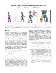
Fig. 1. Algorithm overview. A: input mesh model; B: smoothed curvature directions; C: iso-θ and φ curves. The 

singular vertices, edges and triangles are highlighted; D: chart layout; E: final result, obtained after fixing the 

charts with singularities; F: base complex. 

One of the main achievements of our algorithm is its ability to automatically extract a 

quadrilateral chart layout for the global parameterization. The size (side length) of the 

charts is determined by a user prescribed parameter ω. As demonstrated in Figure 1, the 

extracted charts are well shaped and equally sized. They also have very regular connectivity, 

with mostly valence four vertices. 

Our method can construct a curvature-adapted globally smooth conformal parameterization 

or a quasi-isometric parameterization. In the latter case, the near zero distortion is 

obtained at the expense of introducing more singular points. This tradeoff is achieved by 

an additional processing step that controls the curl of the vector field. 


· 5 

The algorithm for computing our globally smooth parameterizations consists of the following 

four stages. 

—Vector field smoothing (optional): This pre-processing step smoothes the input orthogonal 

curvature vector fields and extrapolates them into isotropic regions of the mesh 

where principal directions of curvature are undefined (Figure 1-B and Section 4.2). This 

procedure is fully stand-alone and can be used not only for periodic parameterization but 

also for other applications that utilize curvature vector fields on meshes (e.g. triangular 

remeshing). 

—Curl-correction (optional): A global isometric parameterization is usually not possible 

without a large number of singular points. As explained in Section 4.1 most of these 

points correspond to regions of non-zero curl in the vector fields. Hence, to reduce the 

number of singular points we introduce an optional procedure that rescales the vector 

fields to reduce the curl as much as possible. The procedure is applied to the input 

vector fields and its results are used as input to the subsequent parameterization step. 

If curl-correction is applied, the resulting parameterizations will remain conformal and 

have far less singular points, but will usually exibit larger stretch. 

Both vector field smoothing and curl correction are optional stages which can be skipped 

by the user if desired. Hence, we prefer to describe those stages in the second part of 

the paper, after the main concept of alternative, periodic variables is introduced in the 

context of parameterization. 

—Parameterization using alternative variables: This is the main step of the algorithm. 

To explicitly account for translational and rotational degrees of freedom in the parameterization 

formulation, we develop an energy functional using alternative variables 

(trigonometric functions of the actual parameterization). The derivations are described 

in detail in Section 2. The derived energy functional (Equation 4) is minimized using 

the numerical procedure described in Section 2.5. Figure 1-C shows the iso-curves of 

the so-computed variables. 

—Extraction of chart layout and chart parameterization: The final stage of the algorithm 

computes the actual surface parameterization given the solution in terms of 

alternative variables (Section 3). In a continuous setting, it is well known that a parameterization 

of a genus g object has at least 2g − 2 singular points, where the derivatives 

of the parameterization vanish. As a consequence, the piecewise linear functions constructed 

by our algorithm exhibit vertices, edges and triangles that do not satisfy the 

requirements of a valid 2D planar triangulation (highlighted in Figure 1-C). Our algorithm 

first extracts the parameterizations for each individual mesh triangle. Then, it uses 

those to define a global chart layout. Then, for each chart, if the chart does not contain 

any singularity, it reconstructs the parameterization in it by assembling each individual 

triangle in parameter space. Otherwise, the chart (that contains singularties) is splitted 

and re-parameterized. The final result and the corresponding base complex are shown in 

Figure 1-C and D respectively. 

The result of the procedure is a global conformal parameterization that is continous 

almost everywhere. The parameterization is aligned with the vector field, which in our 

context is defined by the principal curvature directions on the mesh. If no curl-correction 

is performed, the parameterization is quasi-isometric. 


6 · 

Fig. 2. A Global Parameterization (or manifold) is a set of overlapping parameterizations (ϕ,ϕ ′ ,...) connected 

by transition functions (τ ϕ→ϕ ′ ...). 

Our parameterization can be used for a variety of mesh processing applications. In particular 

in Section 5 we demonstrate the use of the parameterization for curvature-alligned 

quadrilateral remeshing. Given our parameterization, the mesh generation procedure is elegant 

and straightforward. Other possible important applications of our method concern 

smooth surface reconstruction and texture mapping. 

2. PERIODIC GLOBAL PARAMETERIZATION 

2.1 Definition 

We first give the definition of a manifold (also called a global parameterization in our 

context). This notion permits defining a globally smooth parameterization of a surface 

of arbitrary genus, by combining multiple parameterizations of charts extracted from the 

surface and linked by transition functions. To our knowledge, this notion of manifold was 

first used in geometric modelling by Grimm and Hugues [Grimm and Hugues 1995]. More 

recently, a C ∞ class of surfaces based on manifolds was proposed in [Ying and Zorin 2004]. 

Given a surface S, we consider a set of (possibly overlapping) topological disks {C} 

called charts, and a set of functions {ϕ} mapping each chart C to a 2D domain Ω (see 

Figure 2). The coordinates in 2D space will be denoted by θ,φ in what follows 1 . The 

set of functions {ϕ} is called a global parameterization (or a manifold) if it satisfies the 

following condition: 

Given two charts C and C ′ , if their intersection C ∩ C ′ is a topological disk, then the 

images of the intersection C ∩ C ′ in parameter space through ϕ and ϕ ′ are linked by a 

simple geometric transform τ ϕ→ϕ ′: 

∀p ∈ C ∩ C ′ , 

ϕ ′ (p) = τ ϕ→ϕ ′ (ϕ(p)) 

The τ ϕ→ϕ ′ functions are called transition functions. (see e.g. [Khodakovsky et al. 

2003]). Manifolds are called affine if all the transition functions are translations. Complex 

manifolds admit a more general class of holomorphic transition functions, including 

1 we use θ and φ rather than the traditional u,v or s,t to indicate the periodic nature of these coordinates 


· 7 

similarities (i.e. rotation + translation + scaling), see e.g. [Weisstein ] for a definition of 

these classes of objects. Whereas previous work focusses on affine manifolds (see e.g. 

[Gu and Yau 2003; Gortler et al. 2004]), the method we present constructs a sub-class of 

complex manifolds, permitting both translational and rotational degrees of freedom in the 

transition functions. We show the benefit of introducing the additional rotational degree of 

freedom in the applications section. 

As previously mentionned in the introduction, our goal is to construct a global parameterization 

such that the gradients ∇θ, ∇φ of the parameter-space coordinates θ,φ are 

aligned with two prescribed vector fields (for instance, the principal directions of curvature). 

We first start with the simplest possible charts, i.e. the triangles. In our initial setting, 

the global parameterization is defined by the coordinates θi T ,φi 

T at the corners of the triangles, 

where the global index i denotes a vertex, and where T denotes a triangle. Using 

the so-defined manifold structure, it is possible to derive a parameterization of more general 

charts, by assembling all of their triangles in parameter space, as shown further in the 

paper. 

We first consider the case of an affine manifold (i.e. the transition functions τ ϕ→ϕ ′ are 

translations). We will then show how to introduce the rotational degree of freedom. Given 

two triangles T = (i, j,k) and T ′ = (k, j,l) sharing the edge ( j,k), their parameter-space 

coordinates (θ,φ) define an affine manifold if: 

( θ 

T 

j 

φ T j 

) ) (θ T ′ 

j 

− 

φ T ′ 

j 

= 

( 

θ 

T 

k 

φ T k 

) ( 

θ 

T ′ ) 

− 

k 

φ T ′ 

k 

We now need to derive an energy functional F, depending on all the (θi T ,φi T ) coordinates 

and characterizing the alignment of the gradients (∇θ,∇φ) with the principal directions of 

curvatures. In our formulation of the energy functional F, instead of expressing Equation 

1 as a constraint, we will replace the (θi T ,φi T ) variables with alternative variables, associated 

with the vertices (rather than the corners of the triangles), and naturally satisfying 

the constraints. We will then show how to retreive the (θi T ,φi T )’s from those alternative 

variables. 

To do that, we introduce an additional restriction on the transition functions τ ϕ→ϕ ′: the 

coordinates of the translation vectors connecting two charts should be integer multiples of 

2π. With this additional constraint, we have: 

( cosθ 

T 

j 

sinθ T j 

) 

= 

(cos(θ T ′ 

j 

sin(θ T ′ 

j 

) 

+ 2sπ) 

= 

+ 2sπ) 

) (cosθ T ′ 

j 

sinθ T ′ 

j 

; 

( cosφ 

T 

j 

sinφ T j 

) 

= 

) (cosφ T ′ 

j 

sinφ T ′ 

j 

(this condition is also satisfied at vertex k). As a consequence, given a vertex i, for all the 

triangles T incident to i, the values of cosθi 

T and sinθi 

T (resp. φ) coincide. Therefore, 

we introduce the variables U i = (cosθi T ,sinθi T ) and V i = (cosφi T ,sinφi T ), that no-longer 

depend on T (they are attached to the vertices rather than the corners). 

We now consider the more general case of a sub-class of complex manifolds where transition 

functions τ ϕ→ϕ ′ can be combinations of translation and rotation. As previously done, 

we introduce some restrictions: the coordinates of the translations should be multiples of 

2π (as before) and the angles of the rotations should be multiples of π/2. We will refer to 

this configuration as a periodic global parameterization. In this setting, the compatibility 

condition connecting two triangles (Equation 2) is replaced with: 

(1) 

(2) 


8 · 

∃r ∈ {0,1,2,3} 

( cosθ 

T 

) ( ) ) 

r 

j 0 −1 

(cosθ T ′ 

sinθ j 

T j 

= 

1 0 sinθ T ′ 

j 

; 

( cosφ 

T 

j 

sinφ T j 

) 

= 

( 

0 −1 

1 0 

) ) 

r 

(cosφ T ′ 

j 

sinφ T ′ 

j 

(3) 

As a consequence, given a vertex i, for all the triangles T incident to i, the values of 

cosθi 

T and sinθi 

T (resp. φ) coincide up to a change of sign and a swapping of the sine and 

cosine. 

We will now show how to express the alignment with the directions of principal curvatures 

in terms of the variables (U i ,V i ) (Sections 2.2, 2.3, 2.4), then show a procedure to 

retreive the parameter-space coordinates (θi T ,φi T ) from the alternative variables (Section 

3.1). We will then proceed to extract the chart layout (Section 3.3), and show how to retreive 

a parameterization of the charts from the per-triangle (θi T ,φi T ) coordinates (Section 

3.4). 

2.2 Problem Statement 

As described in Section 1.2 the input to our algorithm consists of two orthogonal control 

vector fields ⃗K and ⃗K ⊥ defined on the surface S, and a chart size parameter ω. The meaning 

of this parameter ω and how to choose it is explained below. 

Given the input, our method aims to construct a complex manifold {ϕ T } = {(θ T ,φ T )} 

such that each function ϕ T associated with the triangle T satisfies: 

∇θ T = ω⃗K ; ∇φ T = ω⃗K ⊥ (4) 

In addition, the complex manifold should be a periodic global parameterization, i.e. the 

transition functions τ T →T ′ should be solely composed of translations of multiples of 2π 

and rotations of multiples of π/2. 

The gradient of the parameterization should not depend on the vector fields magnitude. 

When our goal is to construct a parameterization as isometric as possible, we normalize the 

control vector fields ‖⃗K‖ = ‖⃗K ⊥ ‖ = 1. If we want to reduce the curl of the vector field and 

hence minimize the number of singularities in the parameterization, the vector field is first 

normalized and then scaled as described in Section 4.1. This leads to a parameterization 

which remains conformal, but is no longer isometric. 

Due to this normalization, the parameter ω controls the period of the θ and φ functions. 

As described in Section 3.3, we will use the [0,2π] periods of the parameterization to define 

the chart layout. Hence, ω will determine the size of the charts. In all our examples, we 

set ω to ten times the average edge length in the input mesh. Note that if ω is too large, 

charts that are not homeomorphic to disks may be generated. This can be easily detected 

(by computing the Euler-Poincarré characteristic of the charts), and ω can be automatically 

decreased if such a configuration is detected. 

In the general case, Equation 4 has no solution. Since curl(∇ρ) = 0 for any scalar field 

ρ, a solution exists only if curl(⃗K) = curl(⃗K ⊥ ) = 0 [Needham 1994]. In Section 4.1 we 

describe an optional procedure to minimize the curl of the control vector field ⃗K. However, 

to be assured of a solution, we assume that the control vector field might have non-zero 

curl. In this setting, since Equation 4 has no solution in general, we minimize the following 

energy functional instead: 


· 9 

P 3 

P 2 

e 2 

e 1 

K 

y 

x 

P 1 

e 3 

Fig. 3. 

Triangle notations. 

F = 

∫ 

S 

( 

‖∇θ − ω⃗K‖ 2 + ‖∇φ − ω⃗K ⊥ ‖ 2) dS (5) 

Given this problem setting, the main difficulty is to express the alignment of the gradients 

with the control vector field ⃗K independently of the translational and rotational degrees 

of freedom. Since the translation-invariance criterion is the easier one, it will be explained 

first (Section 2.3) and then refined to introduce the rotational degree of freedom (Section 

2.4). 

2.3 Translation-invariant Energy Functional 

The main challenge in the formulation of Equation 5 is finding a way of solving for a periodic 

function. As explained in Section 2.1, to support translational invariance in parameter 

space, we propose to use the 2π periodicity of the sine and cosine functions. As shown 

below, it is possible to restate the alignment with the control vector fields in terms of the 

sines and cosines U = (cosθ,sinθ) and V = (cosφ,sinφ) of the parameters θ and φ. The 

U and V ’s will be the unknowns of our problem. Thus, we will obtain a periodic definition 

of the minimizer of the energy functional F. 

As shown in Appendix A, the following function F ∗ admits the same minimizer as our 

energy function F given Equation 5: 

F ∗ 

= ∑(‖∇θ − ω⃗K T ‖ 2 + ‖∇φ − ω⃗K T ⊥ ‖ 2 )A T (6) 

T 

where A T is the area of triangle T , and ⃗K T and ⃗K T 

⊥ denote the average value of ⃗K (resp. 

⃗K ⊥ ) at the three vertices of the triangle T . We now consider a single entry in this sum: 

F T = (‖∇θ − ω⃗K T ‖ 2 + ‖∇φ − ω⃗K ⊥ T ‖ 2 )A T (7) 

Since it is difficult to derive an expression for F T directly, we will first study F θ T,i , the 

energy along the edges ⃗e i of T (Figure 3) with respect to θ. The energy F φ T,i 

with respect 

to φ is derived in a similar manner. We will then express F T as a linear combination of the 

FT,i θ ’s and Fφ T,i ’s. 


10 · 

K3’ 

K3 

r = 2 

3 

K2 

K 1’ = K 1 

r 

1= 0 

K2’ 

r = 1 

2 

Fig. 4. 

Locally re-orienting the control vector field. 

Intuitively, when moving along the edge⃗e i , Equation 4 dictates that a change in θ should 

depend on ‖⃗e i ‖ and on the angle between⃗e i and ⃗K (it should be proportional to ⃗K.⃗e i ): 

F θ T,i = 

((∇θ − ω⃗K) ·⃗e i 

) 2 

= min s 

{ 

((2sπ + θ i⊕2 − θ i⊕1 ) − ω⃗K ·⃗e i ) 2 } (8) 

where i ∈ {1,2,3} is a local index in T (see Figure 3) and where ⊕ denotes addition modulo 

3. By approximating the angular deviation along the edges by the norm of the difference 

of the sine and cosine vectors, corresponding to order 1 Taylor expansion, we obtain: 

F θ T,i 

where: 

≃ 

( ∥ cos(ω 

∥ U ⃗K ·⃗e 

i⊕2 − 

i ) −sin(ω⃗K ·⃗e i ) ∥∥∥ 

2 )U i⊕1 

sin(ω⃗K ·⃗e i ) cos(ω⃗K ·⃗e i ) 

U i = (cosθ i ,sinθ i ) 

Note that using this formulation, we no longer depend on the translational coefficient s 

(Equation 8). 

With a derivation similar to the one given in Appendix A, since ⃗K and) 

K ⃗⊥ are linear 

along the edges, we can simply replace ω⃗K ·⃗e i with ω/2 

((⃗K i⊕2 + ⃗K i⊕1 ) ·⃗e i . 

Note that theoretically at this point, we can simply minimize ∑ T,i∈1,2,3 (FT,i θ +Fφ T,i 

), which 

corresponds to a discrete, edge-based version of the energy. The resulting method works 

well for regularly sampled surfaces but is sensitive to anisotropic samplings. For this reason, 

we propose in Appendix B a variant of our objective functional that integrates the 

energy over the triangles. This does not require significantly more complex computations 

and improves the result. 

We now have a formulation of F ∗ that supports translational invariance. We proceed to 

introduce rotational invariance into the formulation. 

2.4 Rotation-invariant Energy Functional 

(9) 


· 11 

In general, it is not possible to globally orient a vector field in a consistent 

way (see the circled region). For this reason, as shown below, we 

modify the formulation of the triangle energy (Equation 7) by locally 

reorienting the vector field in the formulation (Figure 4). 

In our formulation, the orientations of the vectors ⃗K 1 , ⃗K 2 and ⃗K 3 at 

the respective vertices of the triangle (Figure 4) are allowed to vary by 

multiples of π/2. Thus, ⃗K 2 (resp. ⃗K 3 ) is aligned with ⃗K 1 by applying 

r 2 rotations of π/2 (resp. r 3 ). 

The rotation is applied simultaneously to the control vector fields (⃗K i ,⃗K i ⊥ ) and to the 

unknowns (θ i φ i ). Note that an odd difference of r i along an edge means swapping the 

unknowns (i.e., connecting θ’s with φ’s). 

To define the objective function F T on the triangles, we use the same approach as in the 

previous section. We first express the deviation F T,i along an edge and then express F T as 

a linear combination of the F T,i ’s as defined by Equation 19. Since the θ’s and the φ’s may 

be coupled, we can no longer separate them. 

Adding rotational invariance, Equation 8 becomes 

F T,i = min 

s,t 

where: 

r i 

( 0 −1 

∥ 1 0 

= argmax 

r ∈ {0,1,2,3} 

) ri⊕2 

( ) 

θi⊕2 

− 

φ i⊕2 

( 

⃗K 1 . 

δ i = ω/2( 

⃗ K ′ i⊕1 + ⃗K ′ i⊕2 

( 

0 −1 

1 0 

) ri⊕1 

( 

θi⊕1 + 2sπ 

φ i⊕1 + 2tπ 

( ) r ) ( ) ri 

0 −1 

K ⃗ 

′ 0 −1 

1 0 i ; ⃗K i = K ⃗ 

1 0 i 

) 

( ) 

·⃗e i ; δi ⊥ = ω/2 K ⃗ 

i⊕1 ′⊥ + ⃗K i⊕2 

′⊥ 

) ( )∥ 

δi ∥∥∥ 

2 

− 

δi 

⊥ 

·⃗e i 

(10) 

As in the previous section, to take the periodicity of the (θ,φ) parameters into account, 

we solve for the sines and the cosines of these parameters. F T,i as a function of the sines 

and cosines (using the same order 1 approximation as in Equation 9) is then given by: 

F T,i ≃ 

⎛ 

⎞ ∥ cosδ i −sinδ i 0 0 

∥∥∥∥∥∥∥ 

2 

M r i⊕2X i⊕2 − ⎜sinδ i cosδ i 0 0 

⎝ 

0 0 cosδi 

⊥ −sinδi 

⊥ ⎟ 

⎠ Mr i⊕1X i⊕1 

∥ 

0 0 sinδi 

⊥ cosδi 

⊥ 

⎛ ⎞ 

⎛ ⎞ 

0 0 −1 0 

⎛ ⎞ cosθ i 

where: M = ⎜0 0 0 1 

⎟ 

⎝1 0 0 0⎠ ; X i = ⎝ U i 

⎠ = ⎜sinθ i 

⎟ 

⎝cosφ i 

⎠ 

0 1 0 0 

V i sinφ i 

(11) 

As in the previous section, we can simply minimize F ∗ = ∑ T,i∈1,2,3 (FT,i θ + Fφ T,i 

), which 

corresponds to a discrete, edge-based version of the energy, or we can plug this expression 

into the triangle energy formulation (Appendix B, Equation 19). The minimizer of F ∗ is 

computed as described below. 


12 · 

2.5 Numerical Solution Mechanism 

To obtain the minimizer of F ∗ , we fix one of the vertices U 1 = (1,0),V 1 = (1,0) and 

minimize F ∗ with respect to all the other variables. Since F ∗ is a quadratic form, this 

means solving a sparse symmetric system. We use the conjugate gradient algorithm with 

Jacobi’s preconditioner. For models with more than 50K vertices, the norms of the U i ,V i ’s 

quickly decrease when we move far away from the fixed vertex, resulting in both weighting 

biases and numerical instabilities. To stabilize the system, we add a (non-linear) penalty 

term, preventing the norms of the U,V ’s from decreasing: 

F ∗∗ = F ∗ ( 

+ ε ∑ (‖Ui ‖ 2 − 1) 2 + (‖V i ‖ 2 − 1) 2) 

i 

This augmented energy functional is minimized using Newton’s algorithm. In our tests, 

ε = 10 −3 gives good results. Convergence, to ∇F ∗∗ < 10 −6 , is reached after no more than 

5 outer-loop iterations for all the models shown in this paper. 

3. PARAMETERIZATION EXTRACTION 

The output of the solution mechanism described in the previous section is a set of U i ,V i 

variables. These variables correspond to the sines and cosines of the unknown θ i ,φ i coordinates 

that define the global parameterization. To construct a global parameterization 

from those U i ,V i variables, we proceed as follows: 

(1) reconstruct a (θ,φ) parameterization in the simplest possible charts, i.e. in each individual 

triangle (Section 3.1), 

(2) detect the singular vertices, edges and triangles (Section 3.2) 

(3) define the chart layout based on the [0,2π] periods of these triangle parameterizations 

(Section 3.3), 

(4) split and re-parameterize the charts that contain singularities (Section 3.4. 

3.1 Per-triangle parameterization 

i ,φi 

T 

Given the U,V variables at the vertices of a triangle T = (i, j,k), finding the θ i ,φ i (resp. 

j,k) coordinates means determining the integer translational (s i ,t i ) and rotational r i degrees 

of freedom. We explicitely determine the values of r,s,t that minimize the edge-energy 

term (Equation 10). 

To fix the global position and orientation of the triangle in parameter space, we set 

the degrees of freedom r i ,s i ,t i of the first vertex i to (0,0,0). Thus, the θ T coordinates 

at vertex i are given by θi 

T = angle(U i ) and φi T = angle(V i ) where angle(U i ) = 

sign(U i,y )arccos(U i,x /‖U i ‖). 

We now assign the coordinates at the two other vertices j and k by determining the 

differences s T e ,te T ,re T of the translational and rotational degrees of freedom along the edge 

e = (i, j) (resp. (i,k),( j,k)), given by s T e = (s T j − sT i ),tT e = (t T j − ti T ) and re T = (r T j − ri T ). 

We first consider the edge (i, j). The computation for the two other edges is obtained by a 

circular permutation of indices (i, j,k). Given the coordinates (θi T ,φi T ) at vertex i and the 

control vector field values (K i ,Ki ⊥ ) and (K j ,K ⊥ j ) at the vertices i, j, Algorithm 1 explicitly 

computes the differences s T e ,te T ,re T , then the values of θ j T and φ j T . 

The algorithm first determines whether the control vector fields undergo a rotation along 

the edge. In this case, we change the correspondence between θ,φ and U,V . For instance 

a rotation of π/2 corresponds to switching U and V . In this case, θ becomes a function 


· 13 

Algorithm 1 Reconstruction of θ,φ along an edge 

propagate from i to j along e = (i, j) : 

// determine and apply rotation r e 

( ( ) r ) 

0 −1 

re T ← argmax r 

⃗K i . K ⃗ 

1 0 j 

r ∈ {0,1,2,3} 

⃗K j ← 

( ) r T 

0 −1 

e 

K ⃗ 

1 0 j ; ⃗K ⊥ j ← 

θ T j ← angle(U T j ) 

φ T j ← angle(V T j ) 

; 

⎛ 

⎜ 

⎝ θ T j 

φ T j 

⎞ 

⎟ 

⎠ ← 

( ) r T 

0 −1 

e 

K ⃗ 

1 0 

⊥ j 

⎛ 

( ) r T 

0 −1 

e 

⎜ 

⎝ θ j 

T 

1 0 

φ j 

T 

// determine and apply translations s,t 

⃗n ←⃗e/‖⃗e‖ ∣ s T ∣∣θ 

e ← argmin 

T 

s i − (π/ω)⃗n · (⃗K i + ⃗K j ) − θ j T + 2sπ∣ 

∣ te T ∣∣φ 

← argmin 

T 

t i − (π/ω)⃗n · (⃗K i ⊥ + ⃗K ⊥ j ) − φ j T + 2tπ∣ 

θ j T ← θ j T + 2s T e π ; φ j T ← φ j T + 2te T π 

⎞ 

⎟ 

⎠ 

of V and φ a function of −U. The algorithm then determines the difference s T e ,te 

T 

translational degree of freedom by explicitely minimizing the edge energy. 

of the 

3.2 Singular vertices, edges and triangles characterization 

Once we have reconstructed the parameterization in each individual triangle, we need to 

check whether these triangles can be assembled in parameter-space in such a way that they 

form a valid planar triangulation. We already know that the solution of the continuous 

version of the equation presents singularities where the derivatives of the solution vanish. 

In our discrete setting, these singularities appear as vertices, edges and triangles that violate 

the conditions of a valid planar triangulation. These singular vertices, edges and triangles 

can be characterized as follows (see e.g., [Sheffer and de Sturler 2001]): 

—singular vertices: a vertex v is singular if the angles at the corners of the triangles 

incident to v do not sum to 2π. In practice, a singular vertex v can also be characterized 

by the fact that applying algorithm 1 to the one-ring neighborhood of v results in an open 

path. 

—singular edges: an edge e = (i, j) is singular if its length in parameter-space mismatches 

with the one of e ′ = ( j,i), 

—singular triangles: a triangle T is singular if applying algorithm 1 to the three edges of 

T results in an open path or if T has a negative signed area. 


14 · 

3.3 Chart layout 

Once we have computed the local parameterization in each triangle T , we construct the 

chart layout. In our setting, the chart boundaries are defined to be the iso-2kπ lines of θ 

and φ. This defines a set of segments in each triangle. We show below that the set of all 

the iso-2kπ lines of θ and φ is invariant under our transition functions. As a consequence, 

the extremities of these independent segments match along the non-singular edges of the 

triangulation, and the segments form continuous polygonal lines. 

—invariance of the set of iso-lines under valid translations : if a triangle T is traversed 

by an iso-2kπ line of θ (resp. φ), this triangle translated by 2sπ will be traversed at the 

same location by the iso-2(k + s)π line of θ (resp. φ). 

—invariance of the set of iso-lines under valid rotations : if a triangle T is traversed by 

an iso-2kπ line of θ (resp. φ), this triangle rotated by π/2 will be traversed at the same 

location by the iso-2(−k)π line of φ (resp. iso-2kπ line of θ). 

Algorithm 2 chart boundaries construction 

compute chart boundaries: 

for each triangle T 

if T is non-singular 

for k ∈ N such that 2kπ ∈ [min T (θ),Max T (θ)] 

Line l ← line of equation(θ = 2kπ) 

Segment S ← l ∩ T //in parameter space 

store S in T 

store the extremities of S in the corresponding edges of T 

end// f or 

for k ∈ N such that 2kπ ∈ [min T (φ),Max T (φ)] 

Line l ← line of equation(φ = 2kπ) 

Segment S ← l ∩ T //in parameter space 

store S in T 

store the extremities of S in the corresponding edges of T 

end// f or 

end//i f 

end// f or 

for each edge e 

merge the segment extremities stored in e that have the same geometric location in 3D 

end// f or 

for each triangle T 

compute the intersections between the edges stored in T 

end// f or 

recursively remove all dangling segments 

Algorithm 2 computes the chart boundaries. In this algorithm, we suppose that each 

triangle can store a list of segments, and each edge can store a list of segment extremities. 

The algorithm computes the individual segments defined by the intersections of the 


· 15 

Fig. 5. Re-parameterizing the charts with singularities. A,B: charts with four corners are re-parameterized using 

mean-value coordinates. C,D: N-sided charts are splitted into quadrilateral charts. 

triangles with the (θ = 2kπ) and (φ = 2kπ) lines. Both the 2D and 3D locations at the 

extremities of the segments are computed. Then, the algorithm merges the extremities of 

the segments along the edges and intersects them in the triangles. Then, all the dangling 

segments are removed (each segment extremity of valence 1 is “nibbled” until an extremity 

of valence higher than 2 is found). 

The parameterization of the charts that do not contain any singularity can be retreived by 

assembling the triangles in 2D space by a classic greedy algorithm (see e.g., [Sheffer and 

de Sturler 2001]). For the other charts, with singularities, we split them and re-parameterize 

them as shown in the next subsection. If needed, the chart boundaries can be inserted into 

the triangulation (e.g., by using our embedded cellular complex data structure [Li et al. 

2005]). 

3.4 Re-parameterization of charts with singularities 

From the (θ,φ) variables, it is not possible to construct a parameterization in the charts 

that contain singularities. Note that it would be possible to split the charts along the separatrices 

of the singularities and fix the parameterization in the singular triangles. However, 

the corresponding algorithm is quite delicate to implement, and might fail under certain 

configurations of singularities. For this reason, we prefer to use the following simple approach: 

—Charts with four vertices are re-parameterized, using the mean value coordinates method 

[Floater 2003] (Figure 5 A and B), 

—N-sided charts are splitted into quads, by inserting a vertex in the center of the chart 

and in the middle of each side of the chart (Figure 5 C and D). The new vertices are 

connected by geodesics, and the mesh is cut along these geodesics (our implementation 

uses [Li et al. 2005]). 

—If desired, the cross-boundary continuity can be improved by locally applying a relaxation 

procedure [Khodakovsky et al. 2003], [Schreiner et al. 2004]. 

In our experiments, only a small fraction (between 2 and 5 %) of the charts contain 

singularities and require this additional processing. 

By combining the Periodic Global Parameterization (section 2) with the reconstruction 

algorithm presented in this section, it is possible to compute a global parameterization of 

a surface. The next section presents optional vector field processing algorithms that can 

improve the result by pre-processing the control vector field. 


16 · 

Fig. 6. Curl-correction applied to an object of revolution. A: the quasi-isometric parameterization presents 

additional singular points (shown as dots) to take into account the diverging vector field; B: the color shows the 

magnitude of the curl-corrected vector field; C: solution obtained with the curl-corrected vector field. 

4. VECTOR FIELD PROCESSING 

This section presents vector field processing algorithms that can be optionally applied to 

the principal directions of curvature prior to the periodic global parameterization. Section 

4.1 shows how to rescale the control vector field to minimize the number of singularities. 

Section 4.2 presents a method to extrapolate anisotropic zones over the isotropic ones, 

where the principal directions of curvatures are undefined. 

4.1 Curl Correction 

In the formulation presented in Section 2, the emphasis was on constructing a parameterization 

as isometric as possible. We therefore used the degree of freedom offered by 

the periodic functions to let singular points appear in the parameterization. Those additional 

singular points correspond to the “branchings” shown in Figure 6. This formulation 

is suitable for many applications, such as 3D paint systems, where parametric distortion 

is the dominant consideration. For other applications, however, the number of singular 

points may be a serious concern. For instance, in quad-dominant remeshing, each branching 

point results in an undesirable T-vertex in the mesh. Hence, for these applications, we 

introduce a pre-processing technique, that scales the vector fields prior to parameterization, 

to minimize the number of singular points. 

As can be seen in Figure 6, the added singular points correspond to additional sources 

(resp. sinks) in regions where the control vector field diverges (resp. converges), shown as 

red dots in the figure. Intuitively, considering that the vector field corresponds to the speed 

of a non-compressible fluid, those additional sources and sinks are necessary to preserve 

the “quantity of matter” in those regions. By “accelerating” the vector field in converging 

regions and “slowing it down” in diverging regions, we can remove these additional sources 

and sinks. 

Given that the singular points are caused by a non-zero curl, our goal is to minimize the 

curl of the control vector fields ⃗K and ⃗K ⊥ . Since in our setting (Section 2.2) the control 

vector fields are normalized, curl can arise only from non-parallel vectors (directional curl). 

As a consequence, eliminating the curl means rescaling the vector field in such a way that 

the modular curl, arising from variations of the norm ‖⃗K‖, cancels the directional curl. 

Note that our problem is different from computing a Hodge decomposition (see e.g., [Tong 


· 17 

et al. 2003]), since we want to preserve the directions of the vector field. 

More formally, given a unit vector field ⃗K defined over a surface S, we want to find 

a scalar field v such that curl(v⃗K) =⃗0. The vectors will become shorter in converging 

regions (v < 1) and longer in diverging regions (v > 1). Note that since ⃗K and ⃗K ⊥ are 

coupled by the relation curl(⃗K) = div(⃗K ⊥ ).⃗N (where ⃗N denotes the normal to S), the same 

scaling v needs to be applied to both ⃗K and ⃗K ⊥ . In terms of complex analysis, this coupling 

can be explained also by the fact that the θ and φ functions determine a complex potential 

of K, which is necessarily a conformal function (see [Needham 1994]). 

We assume that the direction of ⃗K varies linearly over T . In other words, given a local 

orthonormal frame (x,y) of T , we can parameterize the vector ⃗K by the angle γ between 

⃗K and the x axis: ⃗K = (cos(γ),sin(γ)), with γ = ax + by + c (γ varies linearly over T ). 

Replacing ⃗K with this expression yields: 

( 

( 

curl(v⃗K).⃗N = − ∂v 

∂y 

)cos(γ) + va + ∂v 

∂x 

)sin(γ) + vb = 0 

where γ = ax + by + c 

We search for solutions of Equation 12 that are independent of rotations applied to the 

vector field ⃗K, i.e., independent of the constant c. The solutions of the following system of 

PDEs meet this requirement: 

(12) 

{ 

−∂v/∂y + va = 0 

∂v/∂x + vb = 0 

(13) 

Fig. 7. Curl-correction applied to a model with sharp features. Note how all the branching points on the tentacles 

(top) are removed by the curl correction (bottom). 


18 · 

The solutions of Equation 13 have the form v = Ce ay−bx , where C denotes a constant. 

To solve for the values v i of v at the vertices globally, we express the condition satisfied by 

the variations of v: 

log(v) = log(C) + ay − bx 

∇log(v) = ∇(ay − bx) = (−b a) 

We solve for the ṽ i = log(v i )’s using a least squares formulation: 

G(ṽ) = ∑ 

T 

where: 

∥ ⎛ ⎞ 

⎛ 

∥∥∥∥∥ ( ) 

A T J T ⎝ṽ1 ṽ 2 

⎠ 0 −1 

− J 

1 0 T 

⎝ γ ⎞ 

1 

γ 2 

⎠ 

ṽ 3 γ 3 

∥ 

( ) 

y2 − y 

J T = 1/2A 3 y 3 − y 1 y 1 − y 2 

T 

x 3 − x 2 x 1 − x 3 x 2 − x 1 

where (x i ,y i ) are the coordinates of the vertices of T in the local frame. 

Since the solution is independent of a global scaling applied to all the v i ’s, we fix 

tildev 1 = 0 and solve for all the other ṽ i ’s. Then, we compute the scaling coefficients 

v i = exp(ṽ i ), and normalize them by dividing them by Max(v i ). Then we introduce the v i ’s 

in Equation 5: 

∫ ( 

F = ‖∇θ − ωv⃗K‖ 2 + ‖∇φ − ωv⃗K ⊥ ‖ 2) dS 

S 

We proceed to solve for the minimizer of F as described in Section 2.5. 

4.2 Vector Field Smoothing 

To define the control vector fields, we use an approximation of the principal directions 

of curvature (see e.g., [Cohen-Steiner and Morvan 2003]). This enables us to align the 

parameterization with the main features of the surface S. However, in isotropic regions, 

the principal directions of curvature are undefined. As a consequence, the estimation is 

meaningless in regions where the anisotropy (|kmax/kmin|−1) vanishes. To obtain vector 

fields which are well defined everywhere, we introduce a method for extending the directions 

from the anisotropic regions of the surface into the isotropic regions. This method 

can be applied as a pre-processing step of our parameterization algorithm or can be used by 

other applicatins which utilize curvature fields. The method presented in [Hertzmann and 

Zorin 2000] shares some similarities with ours. The main differences are that our variables 

are the sines and cosines of the angles, this removes some non-linearity from the formulation 

and permits faster convergence. Moreover, our method can handle equality modulo 

π/2, π or 2π (as shown below, for a sphere, this creates 8 quarter poles or 4 half-poles or 

two poles respectively). 

To smooth a vector field, we apply a regularized fitting procedure to a set of variables 

α i , corresponding to the direction of ⃗K i . α i is defined as the angle between the vector ⃗K i 

and a reference direction ⃗H i in the projection plane of the vertex i. To obtain a reference 

direction we select an edge⃗e emanating from i and project it to the plane: 

( ) 

⃗H i = normalize −→e − ( 

−→ e · ⃗N i )⃗N i 

ACM Journal Name, Vol. V, No. N, Month 20YY. 

2 

(14) 

(15)

· 19 

Fig. 8. Rattan objects and globally smooth parameterizations modulo 2π (A), π (B) and π/2 (C). A globally 

smooth parameterization modulo 2π/k has poles of index 1/k (red dots). 

where ⃗N i is the normal at i. To smoothly fit the curvature directions, we minimize the 

following enrgy functional: 

R = (1 − ρ)∑|kmax i /kmin i | ∥ αi − α 0 ∥ 2 

i + ρ ∑R T 

(16) 

i 

} {{ } 

T 

} {{ } 

fitting term smoothing term 

where kmax i (resp. kmin i ) is the maximum (resp. minimum) curvature at vertex i. The 

angles αi 

0 are computed from the initial values of the vector field ⃗K at the vertices. The 

user-defined coefficient ρ corresponds to the desired smoothing intensity (in all our examples, 

ρ = 0.8). The smoothing term R T on a triangle T minimizes the variations of α over 

T and is given by: 

R T = ∑λ i R T,i 

where the variation R T,i of α along the edge e i is given by: 

( ) ( )( )∥ R T,i = 

cosαi⊕2 cosβi sinβ 

∥ − 

i cosαi⊕1 ∥∥∥ 

2 

sinα i⊕2 −sinβ i cosβ i sinα i⊕1 (17) 

with: cosβ i = ⃗H i⊕1 · ⃗H i⊕2 ; sinβ i = (⃗H i⊕1 × ⃗H i⊕2 ).N T 

In this equation, β i denotes the angle between ⃗H i⊕1 and ⃗H i⊕2 , and the λ i ’s used to define 

triangle integrals are computed as described in Appendix B, Equation 19. 

As before, angle differences are approximated by the norm of the difference of the 

sine/cosine vectors. The fitting terms (α i − α 0 i )2 are approximated by the squared norm 

‖(cosα i ,sinα i ) − (cosα 0 i ,sinα0 i )‖2 . 


20 · 

Fig. 9. 

Periodic global parameterizations with various genuses. 

We optimize Equation 16 for the unknowns (cosα i ,sinα i ), using the same solution 

mechanism as in section 2.5. We introduce a penalty term that prevents the norm of the 

unknowns from vanishing. Similar to the penalty function in Section 2.5, the penalty term 

evenly distributes the singular points over the surface, as can be seen in Figure 8. 

Given the α i ’s we recompute the vector field ⃗K i = cosα i 

⃗H i + sinα i 

⃗H i × ⃗N i and ⃗K ⊥ i = 

⃗N i × ⃗K i . 

Using the formulation given in Equations 16 and 17, equality between the α i ’s is considered 

modulo 2π. As a consequence, the created singular points are poles. Namely, they 

are points around which the vector field winds once, which corresponds to a 2π rotation. 

To allow rotations of π (or π/2) (half-poles and quarter-poles), it is possible to enforce 

equality modulo π (or π/2) by solving for intermediary variables ˜α i = 2α i (or ˜α i = 4α i ). In 

practice, this simply means dividing all the α 0 i ’s and the β i’s by 2 (resp. 4), then minimizing 

Equation 16, and finally multiplying the α i ’s by 2 (resp. 4). The result on a sphere is 

shown in Figure 8. Either two poles, four half-poles, or eight quarter-poles are obtained 

(the total number of poles weighted by their multiplicity sums to 2g − 2 as predicted by 

the Hopf-Poincaré theorem). As can be seen in Figure 8-C, this property is used by hat 

makers, who prefer using four quarter-poles rather than introducing “branching” singular 

points. In the case of modulo π/2 and modulo π equality, our method is similar to the 

vector field preprocessing described in [Wei and Levoy 2001]. The main difference is 

that our formulation with periodic variables allows the use of efficient numerical solvers. 

In addition, thanks to our global formulation, the numerical solver evenly distributes the 

singular points over the surface. This cannot be done by classic local relaxation procedures. 

5. RESULTS AND APPLICATIONS 

Table I gives deformation statistics and timings for our approach. Note that in the case of 

Sander’s method [Sander et al. 2002], the model was previously cut to make it homeorphic 

to a topological disk [Sheffer and Hart 2002]. Although our setting is more constrained 

than using disk-like topology, our Periodic Global Parameterization method successfuly 

constructs a quasi-isometric parameterization (PGP) and a quasi-conformal one (ccPGP 

for curl-corrected). Figure 9, 10 and 11 show examples with surfaces of various genuses. 


· 21 

Fig. 10. 

Our method applied to the “buffle” data set. 

Implicit Remeshing 

Most previous curvature aligned remeshing methods compute the streamlines of the curvature 

tensor. Those streamlines can be characterized by an ordinary differential equation 

that can be easily solved by an explicit integration scheme (Runge-Kutta). This integration 

is computed either in parameter-space [Alliez et al. 2003] or directly on the surface [Marinov 

and Kobbelt 2004]. The main difficulty with this approach is to evenly distribute the 

streamlines over the surface. In previous work, this was done by using variants of the local 

streamline seeding strategy described in [Jobard and Lefer 1997]. However, the greedy 

nature of this approach results in an uneven placement of the streamlines (see Figure 12 

(Left)). 

The method described in [Dong et al. 2004] is an attempt to design an implicit scheme. It 

shares some common points with our method. The method constructs a harmonic function, 

and extracts a family of streamlines from a set of iso-curves of this harmonic function. 

However, this method requires the user to manually define the singular points, does not 

align the streamlines to the features of the surface, and still requires an explicit integration 

for computing the streamlines along the orthogonal direction. 


22 · 

Fig. 11. 

Quasi-isometric global parameterization of the “David” data set (200K facets). 

Model ♯∆ Algorithm Stretch Shear time 

Horse 20K Gu et al. 6.777 0.07 NA 

PGP 1.07 0.20 45 s. 

ccPGP 1.176 0.12 53 s. 

Bunny 25K Gu et al. 2.65 0.042 NA 

PGP 1.029 0.167 58 s. 

ccPGP 1.14 0.14 1 min. 12 s. 

Bull 34.5K Sander et al. 1.030 0.1558 1 min. 11 s. 

PGP 1.064 0.1774 1 min. 26 s. 

ccPGP 1.209 0.0885 1 min. 35 s. 

Camel 78K Sander et al. 1.053 0.227 3 min. 51 s. 

PGP 1.048 0.1596 5 min. 46 s. 

ccPGP 1.654 0.0711 6 min. 51 s. 

David 200K PGP 1.121 0.2398 17 min. 35 s. 

ccPGP 1.270 0.1310 20 min. 43 s. 

Lion 400K PGP 1.123 0.1728 33 min. 42 s. 

ccPGP 1.425 0.0826 45 min. 18 s. 

Table I. Statistics and timings of our method without and with curl-correction (PGP and ccPGP respectively), 

compared to Gu et al.’s global parameterization and to Sander et al.’s method. 

Fig. 12. Left: explicit remeshing generates an uneven sampling density and gaps. Right: implicit remeshing 

uisng our method generates a more regular sampling. 


· 23 

Fig. 13. Quad-dominant remeshings. Left: remeshing the “lion” dataset with two different resolutions; Right: 

this dataset presents thin features, likely to be missed by explicit (Runge-Kutta) remeshing algorithms. 

In contrast, given a globally smooth parameterization computed by our approach, the 

families of curves in both directions are defined as iso-θ and iso-φ’s. Hence it is straightforward 

to extract them from our global parameterization. For this reason, our approach 

may be qualified as an implicit remeshing method (Figure 12 (Right)). To speed-up computations, 

as done in [Marinov and Kobbelt 2004], we store in each original triangle T 

the list of iso-θ and iso-φ segments contained by T . Examples are shown in Figure 13. 

The “lion” dataset is remeshed with two different resolutions. The “hand” dataset has thin 

features (e.g., the two tubular features in the lower-right part of the image), that fail to be 

captured by the classic explicit streamline integration. 

Conclusions and Future Work 

In this paper, we proposed a new globally smooth parameterization method. The constructed 

parameterization is aligned with the curvature tensor, and a natural quadrilateral 

and regular chart layout is automatically extracted from it. The technique has a wide range 

of possible applications, including remeshing, as demonstrated in the paper. Other possible 

applications include spline fitting, texture synthesis and geometry compressing using geometry 

images and will be described in future papers. Interactivity may be also introduced 

in the method in two different ways : first, least-squares interactive constraining of the 

vector field can be easily introduced into our approach, by removing degrees of freedom 

from the energy functional. Second, to improve the efficiency and the interactivity of the 

method, hierarchical solvers [Aksoylu et al. 2004] are a possible strategy. 


24 · 

Acknowledgements 

We thank the Aim@shape European Network of Excellence and the INRIA ARC GEOREP 

for their support, Pedro Sander and David Gu for the statistics of their methods, Laurent 

Alonso for the proof in Appendix A. We also thank Stanford University, the ENST and 

Sensable for their 3D data sets. 

REFERENCES 

AKSOYLU, B., KHODAKOVSKY, A., AND SCHRODER, P. 2004. Multilevel solvers for unstructured surface 

meshes. Submitted to SIAM J. Sci. Comput.. 

ALLIEZ, P., STEINER, D. C., DEVILLERS, O., LEVY, B., AND DESBRUN, M. 2003. Anisotropic Polygonal 

Remeshing. ACM TOG (SIGGRAPH). 

COHEN-STEINER, D. AND MORVAN, J.-M. 2003. Restricted delaunay triangulations and normal cycle. To 

appear at SOCG. 

DONG, S., KIRCHER, S., AND GARLAND, M. 2004. Harmonic functions for quadrilateral remeshing of arbitrary 

manifolds. Tech. rep. August. 

FLOATER, M. 1997. Parametrization and smooth approximation of surface triangulations. Computer Aided 

Geometric Design 14, 3 (April), 231–250. 

FLOATER, M. S. 2003. Mean value coordinates. CAGD 20, 19–27. 

FLOATER, M. S. AND HORMANN, K. 2004. Surface parameterization: a tutorial and survey. In Advances on 

Multiresolution in Geometric Modelling, M. S. F. N. Dodgson and M. Sabin, Eds. Springer-Verlag, Heidelberg. 

GORTLER, S., GOTSMAN, C., AND THURSTON, D. 2004. One-forms on meshes and applications to 3d mesh 

parameterization. Tech. rep., Harvard University. 

GOTSMAN, C., GU, X., AND SHEFFER, A. 2003. Fundamentals of spherical parameterization for 3d meshes. 

ACM TOG (SIGGRAPH) 22, 358–363. 

GRIMM, C. AND HUGUES, J. 1995. Modeling surfaces of arbitrary topology using manifolds. In SIGGRAPH 

conference proceedings. 

GU, X. AND YAU, S.-T. 2003. Global conformal surface parameterization. In Symposium on Geometry Processing. 

ACM. 

HERTZMANN, A. AND ZORIN, D. 2000. Illustrating smooth surfaces. In SIGGRAPH Conference Proceedings. 

ACM Press/Addison-Wesley Publishing Co., New York, NY, USA. 

HORMANN, K. AND GREINER, G. 2000. MIPS: An efficient global parametrization method. In Curve and 

Surface Design. 

JOBARD, B. AND LEFER, W. 1997. Creating evenly-spaced streamlines of arbitrary density. In Proc. of the 

Workshop on Vis. in Sci. Comp. Eurographics. 

KHODAKOVSKY, A., LITKE, N., AND SCHRODER, P. 2003. Globally smooth parameterizations with low distortion. 

ACM TOG (SIGGRAPH). 

KRAEVOY, V. AND SHEFFER, A. 2004. Cross-parameterization and compatible remeshing of 3d models. ACM 

TOG (Proc. SIGGRAPH 2004). 

LI, W. C., LEVY, B., AND PAUL, J.-C. 2005. Mesh editing with an embedded network of curves. In Shape 

Modeling International conference proceedings. 

MARINOV, M. AND KOBBELT, L. 2004. Direct anisotropic quad-dominant remeshing. In Proc. Pacific Graphics. 

207–216. 

NEEDHAM, T. 1994. Visual Complex Analysis. Oxford Press. 

PRAUN, E., FINKELSTEIN, A., AND HOPPE, H. 2000. Lapped textures. In SIGGRAPH 00 Conf. Proc. ACM 

Press, 465–470. 

SANDER, P., GORTLER, S., SNYDER, J., AND HOPPE, H. 2002. Signal-specialized parametrization. In Eurographics 

Workshop on Rendering. 

SCHREINER, J., PRAKASH, A., PRAUN, E., AND HOPPE, H. 2004. Inter-surface mapping. ACM TOG (Proc. 

SIGGRAPH 2004). 

SHEFFER, A. AND DE STURLER, E. 2001. Parameterization of faceted surfaces for meshing using angle based 

flattening. Engineering with Computers 17, 326–337. 


· 25 

SHEFFER, A. AND HART, J. 2002. Seamster: Inconspicuous low-distortion texture seam layout. In IEEE 

Visualization. 

TARINI, M., HORMANN, K., CIGNONI, P., AND MONTANI, C. 2004. Polycube-maps. ACM TOG (SIGGRAPH). 

TONG, Y., LOMBEYDA, S., HIRANI, A., AND DESBRUN, M. 2003. Discrete multiscale vector field decomposition. 


WEI, L.-Y. AND LEVOY, M. 2001. Texture synthesis over arbitrary manifold surfaces. In SIGGRAPH 2001, 

Computer Graphics Proceedings, E. Fiume, Ed. ACM Press / ACM SIGGRAPH, 355–360. 

WEISSTEIN, E. W. Manifold. 

YING, L. AND ZORIN, D. 2004. A simple manifold-based construction of surfaces of arbitrary smoothness. 


ZELINKA, S. AND GARLAND, M. 2003. Interactive texture synthesis on surfaces using jump maps. In Symposium 

on Rendering. Eurographics. 

A. INTEGRAL OF A PIECEWISE LINEAR VECTOR FIELD 

Given a piecewise linear vector field K and its average value K T on a triangle T , we prove 

that the two energy functionals F T = ∫ T (∇θ − ωK)2 ds and F ′ T = ∫ T (∇θ − ωK T ) 2 ds have 

the same minimizer: 

F T 

= ∫ T (∇θ − ωK)2 ds 

= ∫ T ((∇θ − ωK T ) + (ωK T − ωK)) 2 ds 

= ∫ T (∇θ − ωK T ) 2 + 2 ∫ T (ωK T − ωK) t (∇θ − ωK T )ds + ∫ T (ωK T − ωK) 2 ds 

(18) 

= ∫ T (∇θ − ωK T ) 2 + 2(∇θ − ωK T ) t ∫ T (ωK T − ωK)ds + ∫ T (ωK T − ωK) 2 ds 

The first term of this expression is F T ′ , the second term vanishes (by definition of the 

average value K T ) and the third term does not depend on θ. As a consequence, we have 

F T = F T ′ + constant. Therefore, F T and F T ′ have the same minimizer. 

B. ENERGY INTEGRATED OVER THE TRIANGLES 

The energy F T integrated over the triangle T can be expressed as a linear combination of 

the FT,i θ and Fφ T,i 

edge energies: 

F T = (‖∇θ − ω⃗K T ‖ 2 + ‖∇φ − ω⃗K T ⊥‖2 )A T = ∑ 

3 λ i (FT,i θ + Fφ T,i ) 

where (λ 1 ,λ 2 ,λ 3 ) are the solutions of : 

⎛ 

(e 1,x ) 2 (e 2,x ) 2 (e 3,x ) 2 ⎞⎛ 

⎞ ⎛ ⎞ 

λ 1 1 

⎜ 

⎝ (e 1,y ) 2 (e 2,y ) 2 (e 3,y ) 2 ⎟⎜ 

⎠⎝λ 2 

⎟ 

⎠ = ⎜ 

⎝1 

⎟ 

⎠ 

2e 1,x e 1,y 2e 2,x e 2,y 2e 3,x e 3,y λ 3 0 

The linear system is obtained by expanding and equating both terms of Equation 19. 

Figure 14 compares the results obtained with the edge-based and the triangle-based energy 

on a mesh with a strong anisotropy. 

i=1 

(19) 


26 · 

Fig. 14. A: a meshed torus with a strong mesh anisotropy; B: result of the edge-based PGP: the parameterization 

is influenced by the mesh anisotropy; C: result of the triangle-based PGP: the parameterization solely depends on 

the geometry.

Periodic Global Parameterization - alice - Loria

Create successful ePaper yourself

Delete template?

Save as template?