Lp Centroidal Voronoi Tessellation and its Applications - alice

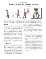
L p Centroidal Voronoi Tessellation and its ApplicationsBruno Lévy ∗Yang Liu ∗AbstractThis paper introduces L p-Centroidal Voronoi Tessellation (L p-CVT), a generalization of CVT that minimizes a higher-order momentof the coordinates on the Voronoi cells. This generalizationallows for aligning the axes of the Voronoi cells with a predefinedbackground tensor field (anisotropy). L p-CVT is computedby a quasi-Newton optimization framework, based on closed-formderivations of the objective function and its gradient. The derivationsare given for both surface meshing (Ω is a triangulated meshwith per-facet anisotropy) and volume meshing (Ω is the interiorof a closed triangulated mesh with a 3D anisotropy field). Applicationsto anisotropic, quad-dominant surface remeshing and to hexdominantvolume meshing are presented. Unlike previous work,L p-CVT captures sharp features and intersections without requiringany pre-tagging.CR Categories: I.3.5 [Computer Graphics]: Computational Geometryand Object Modeling—Geometric algorithms, languages,and systems; AlgorithmsKeywords: Centroidal Voronoi Tessellation, Anisotropic Meshing,quad-dominant meshing, Hex-dominant meshing1 IntroductionMeshing a domain consists in partitioning it into a set of cells thatsatisfy certain geometric requirements specified by the application.∗ INRIA-ALICEe-mail: {Bruno.Levy | Yang.Liu}@inria.frFigure 1: Two applications of L p-CVT. Top left: restricted L p-CVT for anisotropic surface remeshing; right: L p-CVT for hexdominantmeshing.A family of methods, called variational, is based on optimizing anobjective function of the coordinates at the vertices. This familyof methods can efficiently and robustly generate isotropic simplicialmeshes [Du and Wang 2003; Alliez et al. 2005; Tournois et al.2009]. A key ingredient of these methods is the notion of CentroidalVoronoi Tessellation (CVT) [Du et al. 1999] and OptimalDelaunay Triangulation (ODT) [Chen and Xu 2004], used to definethe objective function.This paper deals with generalizing CVT for anisotropic and hexahedralmeshing. Hexahedral meshes are the preferred representationsfor certain finite element simulations and numerical analysis, suchas CFD (computational fluid dynamics), reservoir engineering in oilexploration, or mechanics within highly elastic and plastic domains,for which they provide more reliable simulations while reducing thetotal number of elements. However, meshing with hexahedral ele-

ments is a challenging problem [Shepherd and Johnson 2008]. It isstill performed partly manually and takes several orders of magnitudelonger than meshing with tetrahedra. Designing a hex-meshingalgorithm that is robust, controllable and automatic (see below) isstill an open problem :• robust: A hex-meshing algorithm needs to be independentof the commonly encountered degeneracies and singularities,including non-conforming triangles (or artificial borders), degeneratetriangles, creases and self-intersections;• controllable: Finite Element Modeling applications requirea fine level of control over mesh generation, such as fitting auser-defined background anisotropy field, that specifies boththe orientation and element sizes;• automatic: The algorithm needs to be able to operate on rawdata, without requiring any user input (e.g., tagging features).This paper introduces L p-Centroidal Voronoi Tessellation (L p-CVT), a generalization of CVT well suited to anisotropic, quaddominantand hex-dominant meshing. Like CVT, L p-CVT is basedon a standard Voronoi diagram, but it minimizes a generalized versionof CVT energy that takes into account a predefined backgroundanisotropy field and that favors cubical Voronoi cells. The L p-CVTobjective function and its gradient are computed in closed form forboth surface and volume meshing (i.e., meshing a polygonal surfaceor meshing the interior of a polyhedral domain respectively).After a review of previous work, the paper makes the followingcontributions :• Introduce the definition of L p-CVT and derive the objectivefunction and its gradient in closed-form for surfaces and volumes;• apply restricted L 2-CVT to surface remeshing. Using ananisotropy field oriented along facets normals, L p-CVT reconstructssharp features and self-intersections of the inputsurface without any need to tag them;• apply restricted L p-CVT to feature-sensitive quad-dominantsurface remeshing and 3D L p-CVT to hex-dominant volumemeshing. To the best of our knowledge, this is the first time avariational approach is applied to hex-dominant meshing.2 Background and previous workAnisotropic meshing Several strategies exist for anisotropicmeshing, such as “bubble packing” heuristic [Yamakawa and Shimada2003a], tracing the curvature lines [Alliez et al. 2003], ordirectly minimizing the approximation error [Cohen-Steiner et al.2004]. Labelle and Shewchuk [2003] propose a generalization ofVoronoi diagrams with anisotropy attached to the vertices. Du et al.[2005] propose to generalize the notion of CVT with a continuousanisotropy field. They define Anisotropic CVT and experiment itin 2D. Using the same definition of anisotropy, Valette et al. [2008]propose a discrete approximation operating on a pre-triangulationof the domain. The latter approach shares some similarities withL p-CVT. The differences are (1) that L p-CVT relies on a standardVoronoi diagram (instead of an approximated anisotropic Voronoidiagram), (2) that L p-CVT’s objective function is completely determinedin closed form, allowing for efficient Newton solving insteadof relaxation. This makes it possible to apply L p-CVT to morecomplicated settings (3D surfaces and 3D volumes) and (3) thatL p-CVT can produce quad-dominant and hex-dominant meshes.Quad-dominant surface meshing Directly transforming and optimizingquad-meshes is studied in [Daniels-II et al. 2009]. Bubblepacking, mentioned in the previous paragraph, can be adaptedto optimize quads on surfaces [Itoh and Shimada 2001]. Quaddominantmesh adaption from high-quality triangular meshes isproposed in [Tchon and Camarero 2006; Lai et al. 2008]. Usingthe Morse complex of a Laplacian eigenfunction defines a quadrangulation[Dong et al. 2006; Huang et al. 2008], as well as contouringthe iso-u, v lines of a parameterization [Steiner and Fischer2005; Tong et al. 2006; Kalberer et al. 2007]. Using periodicfunctions and mixed integer optimization avoids the need of predefininga homology basis [Ray et al. 2006; Bommes et al. 2009].However, processing objects with sharp features still requires someconstraints to be defined by the user. In contrast, L p-CVT can reconstructsharp features without requiring the user to tag them.Hex-dominant volume meshing Hex-meshing is an importantand difficult issue, see the survey in [Shepherd and Johnson 2008].Several direct strategies were proposed, such as multiple sweeping[Shepherd et al. 2000], paving and plastering [Staten et al. 2005], oroctree-based methods [Maréchal 2009]. As in surface meshing, itis also possible to contour a volume parameterization [Martin et al.2008], or to use the streamsurfaces of a tensor field [Vyas and Shimada2009]. Indirect methods first construct a tetrahedral meshand transform it into a hex-dominant mesh, using an advancingfront [Owen and Saigal 2000]. The initial tetrahedral mesh can begenerated using “bubble packing” with cubic cells [Yamakawa andShimada 2003b]. The variational hex-dominant meshing methoddescribed here uses a similar workflow, with the difference that itreplaces the “bubble packing” heuristic with the optimization of anobjective function (F Lp ) defined in closed form. This function canbe more efficiently computed and the method scales-up to meshesof industrial size.The remainder of the paper is organized as follows. The next pagraphreviews the notion of CVT (Centroidal Voronoi Tessellation).Section 3 introduces L p-CVT, and Section 4 explains how to computeit. Section 5 demonstrates how L p-CVT allows improvingthe robustness, controllability and automatic behavior of featuresensitivesurface remeshing, quad-dominant surface remeshing andvariational hex-dominant meshing.Centroidal Voronoi Tesselation Centroidal Voronoi Tessellation(CVT) is defined as the minimizer of the objective function F , referredto as the CVT energy :F (X) = F ([x 1, x 2, . . . x n]) = ∑ ∫‖y − x i‖ 2 dyiΩ i ∩Ωwhere Ω i denotes the 3D Voronoi cell of vertex x i, and Ω denotesthe domain to be meshed. Ω can be either a surface (surface meshing),or the interior of a closed surface (volume meshing).The gradient of F is given by [Iri et al. 1984] :∇ F | xi (X) = 2m i(x i − g i) (1)where m i and g i denote the volume and centroid of Ω i ∩ Ω.To minimize F , Lloyd’s algorithm [1982] iteratively moves all thepoints x i at the centroid of their Voronoi cells g i. To improvethe speed of convergence, Du and Emelianenko [2006] solve forthe fixed point of Lloyd’s iteration (∀i, x i = g i) using Newton’smethod for systems of non-linear equations . Since F is of classC 2 [Liu et al. 2009], the speed of convergence can be furtherimproved by directly optimizing F with Newton’s minimizationmethod. To avoid costly evaluation of the Hessian at each iteration,quasi-Newton BFGS can be used instead, requiring only theevaluation of F and its gradients given in Equation 1.

To define a variant of F that admitsconfiguration (3-B) or (3-C) as a stable critical point, intuitivelywe could replace theL 2 norm with the L ∞ norm,since its iso-contours are squares(resp. cubes in 3D). However,the L ∞ norm is not differentiable.The L p norm is a goodapproximation, and easier to manipulatealgebraically as shownfurther.3.1 DefinitionL p Centroidal Voronoi Tesselation (L p-CVT) is defined as the minimizerof the L p-CVT objective function F Lp , obtained by injectingboth the anisotropy term and the L p norm into CVT energy :F Lp (X) = ∑ ∫‖M y[y − x i]‖ p pdy (2)iΩ i ∩ΩFigure 2: CVT energy with anisotropy (A) does not take into accountthe axes if they have the same length (B). This motivates thedefinition of a new objective function (C).3 L p Centroidal Voronoi TessellationThe aim of this paper is to propose a new objective function (F Lp )well suited to variational quad-dominant and hex-dominant meshing,controlled by a given anisotropy field. We make two remarksregarding the classical CVT that motivate our approach :• First, as illustrated in Figure 2, if the axes of anisotropy havedifferent lengths, anisotropic CVT energy can take them intoaccount (2-A), but is not affected by them if they have thesame length (2-B). This motivates generalizing CVT in a waythat can take a directional-only anisotropy into account (2-C).• Second, the “honeycomb” pattern shown in Figure 3-A is notthe only critical point of CVT energy. Regular square andrectangle lattices (3-B,C) are also Voronoi diagrams that arecritical points of CVT energy, since the vertices correspondto the centroids of their Voronoi cells. However, the criticalpoints are unstable (saddles), which means that starting from(3-B) or (3-C), a small perturbation leads to a configurationsimilar to (3-A). As a consequence, CVT is not likely to convergeto (3-B) or (3-C).Figure 3: A: a stable critical point of the CVT objective functionF . B,C: two unstable ones. The contoured value is the L 2 norm.where ‖.‖ p denotes the L p norm (‖V‖ p = p√ |x| p + |y| p + |z| pand ‖V‖ p p = |x| p + |y| p + |z| p ). For an even value of p,‖V‖ p p = x p + y p + z p . The domain Ω is either a surface S (surfacemeshing, see sections 5.1,5.2,5.3), or the interior of a closedsurface S (volume meshing, see section 5.4). An L p CentroidalVoronoi Tessellation (L p-CVT) is a stable critical point of F Lp .The next section presents an algorithm that minimizes F Lp in thegeneral case, with S defined as a piecewise linear complex (PLC),for both surface and volume meshing.If the anisotropy is defined as a symmetric tensor field G y, thematrix M y is obtained from the SVD of G y: M y = Σ 1/2 W andG y = W t ΣW = M t yM y (the columns of M y are the axes ofthe anisotropy ellipsoid).3.2 RemarkBefore explaining how to minimize F Lp , it is interesting to takea close look at the relation between the gradient of the standardCVT energy F and the centroids of the Voronoi cells. Consider theintegration F Ω 0iof CVT energy over a fixed Voronoi cell Ω 0 i and itsgradient :∇| xi F Ω 0i= ∇| xi∫Ω 0 i‖y − x i‖ 2 dy= ∫ ∇|Ω 0 xi ‖y − x i‖ 2 dyi( ∫= 2 xΩ idy − ∫ )ydy0iΩ 0 i= 2m i(x i − g i)Detailed derivations [Iri et al. 1984] show that this result still holdswhen Ω 0 i is replaced with a variable domain Ω ∩ Ω i, that dependson x i. This is because the terms of F that depend on the variationsof the integration domains Ω ∩ Ω i cancel-out when considering theinfluence of two neighboring Voronoi cells. This is no longer true inthe anisotropic case, because of the anisotropy that varies betweentwo adjacent cells. Therefore, to compute ∇F Lp , it is not accurateto replace the centroid g i and mass m i by their anisotropic counterpartsin Equation 1 since doing so ignores the variations of thedomains Ω i. In the general case, the gradient cannot be defined interms of m i, g i and needs to be directly derived from the expressionof F Lp . This motivates the closed form derivations explainedin the next section.

Figure 4: Structure of the integration simplices (white triangle) forsurface meshing, obtained from the restricted Voronoi diagram.4 Computing L p -CVTGiven a domain Ω and a set of points X, computing L p-CVT meansminimizing the function F Lp . We use BFGS, a quasi-Newton algorithm.BFGS needs to evaluate F Lp and its gradient ∇F Lp for aseries of X. For each iteration, the algorithm operates as follows :• The domain Ω is decomposed into a set of simplicial cellson which the expression of F Lp is simple (see Section 4.1),represented by a list of integers;• from this combinatorial representation, the value of F Lp andits gradient ∇F Lp is obtained in closed form (Section 4.2).4.1 Combinatorial Structure of F Lp (X)A Piecewise Linear Complex (PLC) is a set of (possibly nonconvex)polygonal facets, described by their vertices p j and by theirsupport planes (N f , b f ) of equations N f x + b f = 0. The structureof the algorithm is the same for surface meshing (remeshing aPLC) and volume meshing (meshing the interior of a closed PLC).Determining the combinatorial structure of F Lp means decomposingΩ into simple cells, called integration simplices, on which F Lpcan be expressed in function of the variables x i and the parametersp j, (N f , b f ).Surface meshing: The combinatorial structure of F Lp is determinedby the restricted Voronoi diagram (RVD), i.e. the intersectionbetween the 3D Voronoi cells and the surface S (colored polygonsshown in Figure 4). The RVD is first computed by an exactalgorithm [Yan et al. 2009]. Then, each restricted Voronoi cellΩ x0 ∩ S is decomposed into a set of triangles. Figure 4 shows oneof these triangles highlighted in white, with vertices C 1, C 2, C 3;Figure 6: Structure of the integration simplices (white tetrahedron)for volume meshing, obtained from the clipped Voronoi diagram.In surface meshing, the vertices C i can have three different configurations,i.e., three different expressions of them in terms of thevariables and parameters (see also Appendix B.2) :• A (blue): a vertex p j of S.• B (green): intersection of one bisector [x 0, x i] and two facets(N f , b f ), (N g, b g) of S;• C (red): intersection of two bisectors [x 0, x i], [x 0, x j] and afacet (N f , b f ) of S ;Volume meshing: the combinatorial structureis determined by the clipped Voronoi diagram,i.e. the intersection between the 3D Voronoi cellsand the interior of the closed surface S (coloredpolyhedra shown in Figure 6). These 3D clippedVoronoi cells are obtained by starting from theirfaces lying on S, i.e. the Restricted Voronoi Diagram(Figure 5-A). The next step computes the”walls”, i.e. the clipped faces of the 3D Voronoicells, shown in Figure 5-B. The ”walls” are constructedby turning around the cells of the restrictedVoronoi diagram (blue lines on the oppositeillustration) and the faces of the Voronoi cells(black lines), alternating each time a vertex of configuration (C)is crossed (in red). The resulting clipped Voronoi cells are closed(Figure 5-C) by a greedy propagation over the Delaunay graph.Then, inner cells are obtained (Figure 5-D), also by a greedy propagationover the Delaunay graph. Finally, each cell Ω x0 ∩ int(S)of the clipped Voronoi diagram is decomposed into tetrahedra. Oneof them, with vertices x 0, C 1, C 2, C 3, is highlighted in white inFigure 6.Compared with surface L p-CVT, there is an additional possibleconfiguration for a vertex C i:• D (yellow): Voronoi vertex, determined by the intersection ofthree bisectors [x 0, x i], [x 0, x j], [x 0, x k ];At this stage, the combinatorial structure is determined, representedby a list of 10 integers per integration simplex x 0, C 1, C 2, C 3 :the first integer is the index of x 0, and three integers per vertex Cencode the configuration of vertex C. A positive integer k denotesthe bisector [x 0, x k ] and a negative integer k corresponds to theboundary plane (N −k , b −k ). The implementation is provided inLpCVT/combinatorics, in the supplemental material.4.2 Algebraic Structure of F Lp (X)Figure 5: Computing the clipped Voronoi diagram (see also video).Some facets/cells were removed to reveal the internal structure.The energy F Lp and its gradient ∇F Lp are computed from the combinatorialstructure (array of integers), the array of vertices (x i) andthe array of boundary planes (N f , b f ), by summing the contributionsF T L pand ∇F T L pof each integration simplex T . The remainderof this section and the Appendix detail this computation.

Expression of F LpThe integration F T L pof the L p energy over an integration simplexT is given by :FL T p= ∫ ‖M T (y − x 0)‖ p p dyTwhere:⎧⎪⎨⎪⎩=|T |( n+pn )∑α+β+γ=pU α 1 ∗ Uβ 2 ∗ Uγ 3U i = M T (C i − x 0)V 1 ∗ V 2 = [x 1x 2, y 1y 2, z 1z 2] tV α = V ∗ V ∗ . . . ∗ V(α times)V = x + y + zIn surface meshing, T denotes the triangle T (C 1, C 2, C 3)and n = 2. In volume meshing, T denotes the tetrahedronT (x 0, C 1, C 2, C 3) and n = 3.Proof: see Appendix A.(3)Figure 8: Remeshing the ’block’ dataset. Left: with standard CVTenergy. Right: L 2-CVT with normal anisotropy recovers the features,without needing pre-tagging or constrained optimization.Expression of ∇F LpThe gradient of F T L prelative to X is obtained by the chain rule :dF T (x0, C1, C2, C3)LpdX= dF T Lp+ dF T Lp dC 1dx 0 dC 1 dX + dF T Lp dC 2dC 2 dX + dF T Lp dC 3dC 3 dXwhere dA/dB = ( ∂a i /∂b j ) i,jdenotes the Jacobian matrix of Awith respect to B. See Appendix B for the detailed derivations. Themultithreaded implementation is provided in LpCVT/algebra,in the supplemental material. The thorough analysis of the continuityof F Lp will be addressed in a future publication. Experimentally,BFGS applied to F Lp behaves well (does not oscillate).5 ApplicationsWe shall now present some applications to surface remeshing andvolume meshing. All tests were performed on a 8-cores, 2.2 GHzcomputer running the multithreaded implementation (Section 4).5.1 Anisotropic Surface RemeshingThe simplest application of L p-CVT is anisotropic surface meshing(p = 2). As a generalization of [Yan et al. 2009] to the anisotropicsetting, anisotropic L 2-CVT can be used to remesh a surface withprescribed anisotropy. The surface meshing framework is used, i.e.F Lp is minimized on the restricted Voronoi diagram. Each facet fhas an associated anisotropy M f , defined as a smoothed estimate ofthe curvature tensor [Ray et al. 2006]. Typical examples are shownin Figures 7 and 1.Figure 7: Remeshing an ellipsoid with anisotropic L 2-CVT. Verticesare aligned along the principal curvature lines.Figure 9: Left: ’mazewheel’ dataset (borders shown in red); Right:isotropic remesh and angles histogram. Timing: 132 seconds.5.2 Fully Automatic Feature-Sensitive RemeshingRemeshing surfaces with features is a challenging problem. Existingapproaches [Tournois et al. 2009; Yan et al. 2009] let the userspecify which edges correspond to features, and use constrained optimizationto sample them properly. For mechanical parts, it may betedious to select the feature edges by hand (see e.g. Figure 9). Witha specific definition of per-facet normal anisotropy, the L p-CVT objectivefunction naturally recovers the features, without needing totag them or using any expensive constrained optimization. The normalanisotropy M f associated with facet f is defined as follows :⎛ ⎞M f = (s − 1) ⎝ Nf x[N f ] tN f y[N f ] t ⎠ + I 3×3N f z [N f ] twhere N f denotes the unit normal of facet f and s the importanceof normal anisotropy (s = 5 in the results herein). Applying M fto a vector v magnifies the component of v aligned with N f by afactor of s. In other words, normal anisotropy penalizes the verticesthat are far away from the tangent plane of the surface. On a sharpedge e, the combined effects of the anisotropies of both facets incidentto e tend to attract vertices onto e. Figures 8,9,10 show someexamples, statistics and timings.To ensure the remesh is homeomorphic to the initial surface, itis sufficient to satisfy the Topological Ball Property [Edelsbrun-

Figure 10: Left: ’nastycheese’ dataset (borders shown in red);Right: isotropic remesh and angles histogram. Bottom: closeup.Sharp features are naturally reconstructed by L 2-CVT with normalanisotropy, without needing to detect or tag them. Timing: 215 s.Figure 11: Thin features create restricted Voronoi cells with severalconnected components. A: this results in sheets of non-manifold triangles;B: the dual of the connected components of the RVD recoversthe correct topology, with two sheets of triangles.ner and Shah 1997], i.e. each restricted Voronoi vertex/edge/faceshould be homeomorphic to a point/segment/disc. This property isa special case of the nerve theorem, also valid for any partition ofthe original surface. For restricted Voronoi cells that have multiplecomponents, we consider each component as an independentcell and compute the dual of the so-defined partition. Consideringthe connected components as individual cells properly recoversthin features. After separating the connected components, if somerestricted Voronoi faces are still not homeomorphic to disc (e.g.cylinders), topology control [Yan et al. 2009] is performed, i.e. interleavedDelaunay refinement and optimization of F L2 . Figure 11shows a detail of the ’nastycheese’ surface, with such non-manifoldconfigurations resolved by the method.Configurations with non-conforming, self-intersecting surfaces canalso be handled by normal anisotropy. The intersections curves donot need to be computed explicitly, they are naturally reconstructedby the L 2-CVT framework with normal anisotropy, for the samereason as sharp features mentioned above. On an intersection, thecombined anisotropies of both sheets place vertices on the intersectioncurve, that appears in the remesh as non-manifold edges, shownin red in Figure 12. A CAD dataset is shown in Figure 12-bottom.The remeshing framework fixes the gaps (artificial borders shownin red) and samples intersection curves without any pre-processingor manual intervention.Figure 13 compares the result with the method developed by Deyet al. [2008] based on Delaunay refinement and protecting balls.Delaunay refinement has the advantage of providing a solid mathematicalfoundation that helps proving that the remesh is isotopicto the original surface, and that the pre-determined creases are recovered.In our case, using the connected components of the RVDand topology control ensures that the remesh is homeomorphic tothe initial surface. As a variational method, L 2-CVT globally optimizesthe vertices locations, resulting in nearly equilateral trianglesof homogeneous sizes.Figure 12: Remeshing surfaces with self-intersections. L 2-CVTwith normal anisotropy naturally samples the intersections.

Figure 13: Comparison with Delaunay refinement [Dey and Levine2008] (data kindly provided by paper’s author). L 2-CVT timing:236 seconds (8 cores, 2.26 GHz).However, since creases are not tagged, we cannot prove thatanisotropic L 2-CVT faithfully recovers them in all possible cases.To show the robustness and practical value of L 2-CVT, further testsare provided in the supplemental material (images and meshes) ona variety of meshes with unconformities (artificial borders, creases. . . ). Studying how L 2-CVT behaves from the point of view ofε-sampling generalized to non-smooth surfaces [Boissonnat andOudot 2006] may yield theoretical guarantees, but this may be difficultto achieve with a variational method that moves all the vertices.5.3 Variational Quad-Dominant Surface RemeshingAs discussed in Section 3, L p-CVT can be applied to quaddominantsurface meshing. Using a value of p that is sufficientlylarge gives a good approximation of the L ∞ norm (p = 8 in theresults herein). Figure 14 shows an example of quad-dominantremeshing, using L 8-CVT. An estimate of the principal directionsof curvatures [Ray et al. 2006] is used to steer the orientation ofthe quads. The normal vector is scaled by 5, to ensure that sharpfeatures are reconstructed (see previous subsection). We performinterleaved refinement / optimization of F Lp iterations, as done in[Tournois et al. 2009] :(1) distribute vertices randomly(2) optimize F L8(3) for each refinement iteration(4) insert a new vertex at the center of each edge of the RDT(5) optimize F L8(6) compute the Restricted Delaunay Triangulation(7) merge triangles in priority orderRefinement for quad meshes (step 4) consists in inserting a vertexin the middle of each edge of the restricted Delaunay triangulation.Finally, the quad-dominant remesh is extracted from the restrictedDelaunay triangulation (Figure 14 top left) by merging pairs of triangles,sorted by the angle at the corners of the so-obtained quads(Figure 14 top right). The result is compared with [Ray et al. 2006]and the most recent [Bommes et al. 2009] quad-remeshing methods.The strong point of [Bommes et al. 2009] is the ability of generatinga nearly regular quad-only mesh, well suited to Splines fitting.The advantages of L p-CVT are the fact that it is fully automatic,and the smaller variations in angles and edge lengths, suitable fornumerical simulations that rely on homogeneous element sizes.Besides orientation of the elements, the anisotropy matrix M f associatedwith each facet f can also prescribe element sizes (by scalingthe axes, i.e., the columns of M f ), as shown in Figure 15. Inthis example, an approximation of local feature size is used to generatesmaller elements in curved and thin zones. If a different scalingfactor is applied to each anisotropy axis, then an anisotropicrectangle/triangle mesh is obtained (see Figure 16). In this example,the used anisotropy is an approximation of the curvature tensor.Figure 14: Variational Quad-Dominant Remeshing of the ‘fandisk’dataset and comparison with previous work (data kindly providedby paper’s author). L p-CVT timing: 322 seconds.Figure 15: Variational Quad-Dominant Remeshing of the ‘chineselion’ dataset with varying element sizes. Timing: 412 seconds.Figure 16: Variational Quad-Dominant Remeshing of the ‘Stanfordbunny’ dataset with anisotropic elements. Timing: 271 seconds.

Figure 17: Variational Hex-Dominant Meshing and comparison with [Maréchal 2009] (data kindly provided by paper’s author).5.4 Variational Hex-Dominant MeshingOur framework extends naturally tovariational hex-dominant meshing. Thevolume framework is used (i.e., L p-CVT is computed on the clippedVoronoi diagram), with an anisotropymatrix M associated with each integrationsimplex. The anisotropy isattached to the facets of the surface,defined as in the previous section,and each integration simplex uses theanisotropy M f of the facet f nearestto its centroid, queried using ApproximatedNearest Neighbor [Mount andArya 1997]. Note that the Delaunay triangulationrestricted to the interior ofS is smaller than the interior of S, asshown in the opposite figure. To avoidthis “shrinkage”, vertices on the boundaryrequire a special treatment, similarlyto [Tournois et al. 2009]. Vertices on the boundary are computedby the surface framework, as in the previous subsection, usingthe same values of M f . These vertices are characterized by aFigure 18: Mesh repair, comparison with Delaunay refinement[Busaryev et al. 2009], (data kindly provided by paper’s author).non-empty intersection of their Voronoi cells with the surface S.After the optimization step, the algorithm computes the Delaunaytriangulation of the vertices restricted to the interior of S, using thecombinatorial information computed in Section 4.1. Each vertex ofconfiguration D (Voronoi vertex inside S) corresponds to a tetrahedron.Finally, the tetrahedra are merged to form hexes, using combinatorialoptimization [Meshkat and Talmor 2000]. The subgraphsof the simplex graph that correspond to hexes are pattern-matchedand hexes are generated, in priority order, determined by dihedralangles and face planarity.Figure 17 shows a hex-dominant mesh (boundary and crosssections)of a CAD model with timing and stats, and compares theresult with an octree-based method [Maréchal 2009]. The advantageof the octree-based method are that it generates a pure hexahedralmesh with a nearly regular pattern and that it is fast. Theadvantages of L p-CVT is that boundaries are well respected regardlesstheir orientation, and that it generates homogeneous elementsizes. Figures 1 and 19 show examples with smooth surfaces.5.5 Discussion - LimitationsL p-CVT is robust to T-junctions and artificial borders (see the empiricalresults in the paper and supplemental material), i.e. meshesthat have a correct geometry but a non-conforming discretization.However, L p-CVT might not handle properly models that are geometricallyinconsistent. Figure 18 compares the result with theCAD model repair algorithm proposed in [Busaryev et al. 2009] andillustrates this limitation of L p-CVT. The input data has some gaps.L p-CVT misses triangles when a Voronoi edge passes through agap (more triangles are missed when the number of vertices is increased).In practice, hole filling heuristic fixes the problem in mostcases. More formally, we think that the ε-sampling formalism andits extensions [Boissonnat and Oudot 2006] provide a mean of developingthe theoretical tools to study how to recover the missingtriangles with theoretical guarantees. Note also that the continuityof F Lp remains to be studied. Finally, we also mention that underextreme anisotropy (100x ratio between the lengths of axes) convergencebecomes much slower because of the conditioning of theHessian of F Lp .

Figure 19: Variational Hex-Dominant Meshing of the ’dragon’ dataset. Timing: 23 minutes.AcknowledgmentsBExpression of ∇FThis project is supported by the European Research Council(GOODSHAPE ERC-StG-205693). The authors want to warmlythank Rhaleb Zayer and Wenping Wang for many discussions,Jean-François Remacle for help with GMSH, Nicolas Saugnier forparallelization, Dong-Ming Yan for the implementation of RVD,the CGAL project for Delaunay triangulation, Loic Marechal andPierre alliez for data and discussion, Tamal Dey for data and helpwith DelPSC, David Bommes, Leif Kobbelt and Aim@Shape fordata, and the anonymous reviewers for their suggestions that helpedimproving the paper.AProof:Expression of F Lpwhere:F T L p=⎧⎪⎨⎪⎩=∫T (x 0 ,C 1 ,C 2 ,C 3 )|T |( n+pn )∑α+β+γ=p‖M T (y − x 0)‖ p p dyU α 1 ∗ Uβ 2 ∗ Uγ 3} {{ }E T LpU i = M T (C i − x 0)V 1 ∗ V 2 = [x 1x 2, y 1y 2, z 1z 2] tV α = V ∗ V ∗ . . . ∗ V(α times)V = x + y + zThe change of variable x := M T (y − x 0) gives :F T L p=∫T (0,U 1 ,U 2 U 3 )x p dxwhere the integrand is a homogeneous polynomial. The integrationof a homogeneous polynomial of degree p over a simplex ∆ ofdimension n [Lasserre and Avrachenkov 2001] is given by :∫H p(x, x . . . x) =∆n( |∆|n+p )n∑0≤i 1 ≤i 2 ...≤ip≤nH p(x i1 , x i2 . . . x ip )where H p denotes the polar form of the polynomial. SubstitutingH p with x 1 ∗ x 2 ∗ . . . ∗ x p gives the result. □(4)The gradient of F is obtained by combining the gradient of F relativeto the vertices of the integration simplices (Appendix B.1) withthe gradients of Voronoi vertices (Appendix B.2) using the chainrule.B.1 Expression of dF T L pdF T Lpdx 0 U 1 U 2 U 3We first deriveand then dC i. Recalling that F TdX L p=|T |EL T pwhere EL T pis given Equation 4 in Appendix A, we obtain :dF T L p= d(|T | E T L p) = E T L pd|T | + |T |dE T L pdE T LpdU 1 U 2 U 3=⎡⎢⎣∑αU α−1α+β+γ=p;α≥1∑βU1αα+β+γ=p;β≥1∑γU1αα+β+γ=p;γ≥1In surface meshing, |T | = 1/2 ‖N‖ and :⎤1 ∗ U β 2 ∗ U γ 3∗ U β−12 ∗ U γ 3⎥∗ U β 2 ∗ U γ−1 ⎦3d|T |dU 1 U 2 U = 3( −12|T | [N × (U2 − U 3)] t [N × (U 3 − U 1)] t [N × (U 1 − U 2)] t)In volume meshing, |T | = 1/6 U 1 · (U 2 × U 3), and :d|T |= 1/6([U 2 × U 3] t [U 3 × U 1] t [U 1 × U t) 2]dU 1U 2U 3Finally, the derivatives of F T L pwith respect to x 0, C 1, C 2 and C 3are given by :dF T LpdC i= dF T LpdU iM T ;dF T Lpdx 0= − dF T LpdC 1− dF T LpdC 2t− dF T LpdC 3

B.2 Gradients of Voronoi verticesThe gradient of a circumcenter C relative to the four vertices of thetetrahedron is given by :config. B: 1 bisector [x 0x 1] and two planes (N 1, b 1), (N 2, b 2)dC =([x 1 −x 0 ] t) −1 ( )[C−x0 ] t [x 1 −C] t[N 1 ] t[C−x 0 ] t 0[N 2 ] t 0 0config. C: 2 bisectors [x 0x 1], [x 0x 2] and 1 plane (N 1, b 1)dC =([x 1 −x 0 ] t[x 2 −x 0 ] t[C−x 0 ] t 0 [x 2 −C] t) −1 ([C−x0 ] t [x 1 −C] t 0[N 1 ] t 0 0 0config. D: 3 bisectors [x 0x 1], [x 0x 2], [x 0x 3]dC =Proof:([x 1 −x 0 ] t) −1 ([x 2 −x 0 ] t[x 3 −x 0 ] t))[C−x 0 ] t [x 1 −C] t 0 0[C−x 0 ] t 0 [x 2 −C] t 0[C−x 0 ] t 0 0 [x 3 −C] tWe show the result for configuration D (circumcenter of Delaunaysimplex). The result for configurations B and C is obtained similarly.Configuration A, i.e. original vertex of S, yields no derivativesince it does not depend on the x is. In configuration D, the pointC is the circumcenter of the Delaunay simplex T (x 0, x 1, x 2, x 3),obtained by intersecting three bisectors [x 0x 1], [x 0x 2], [x 0x 3] :⎛[x 1 − x 0] t ⎞⎛x 2 1 C = A −1 B where A = ⎜[x 2 − x 0] t⎟⎝⎠ ; B = 1 − ⎞x2 0⎜x 2 22 ⎝− x2 0⎟⎠[x 3 − x 0] t x 2 3 − x2 0We first recall some matrix derivation rules [Minka 1997]:(1) d(AB) = dAB + AdB(2) d(A −1 ) = −A −1 (dA)A −1Using first (1) then (2), the expression of dC can be expanded :dC = d(A −1 B) = (dA −1 )B + A −1 dB= −A −1 (dA)A −1 B + A −1 dB= A −1 (dB − (dA)C)then (dB − (dA)C) is substituted with :⎛⎞−x t 0 xt 1 0 0dB = ⎝ −x t 0 0 xt 2 0 ⎠ ; (dA)C =−x t 0 0 0 xt 3which gives the result. □()−C t C t 0 0−C t 0 C t 0−C t 0 0 C tThe equations for configurations C and B are obtained by replacingthe equations of the last (resp. the last two) bisectors with theequations of a constant plane N t 1C+b 1 = 0 (resp. N t 2C+b 2 = 0).ReferencesALLIEZ, P., COHEN-STEINER, D., DEVILLERS, O., LÉVY, B.,AND DESBRUN, M. 2003. Anisotropic polygonal remeshing.ACM Transactions on Graphics 22, 3, 485–493.ALLIEZ, P., COHEN-STEINER, D., YVINEC, M., AND DESBRUN,M. 2005. Variational tetrahedral meshing. ACM Transactionson Graphics 24, 3, 617–625.BOISSONNAT, J.-D., AND OUDOT, S. 2006. Provably good samplingand meshing of Lipschitz surfaces. In SCG ’06: Proceedingsof the twenty-second annual symposium on Computationalgeometry, 337–346.BOMMES, D., ZIMMER, H., AND KOBBELT, L. 2009. Mixedintegerquadrangulation. ACM Transactions on Graphics 28, 3,1–10.BUSARYEV, O., DEY, T. K., AND LEVINE, J. A. 2009. Repairingand meshing imperfect shapes with Delaunay refinement. InSPM ’09: 2009 SIAM/ACM Joint Conference on Geometric andPhysical Modeling, 25–33.CHEN, L., AND XU, J. 2004. Optimal Delaunay triangulations.Journal of Computational Mathematics 22, 2, 299–308.COHEN-STEINER, D., ALLIEZ, P., AND DESBRUN, M. 2004.Variational shape approximation. ACM Transactions on Graphics23, 905–914.DANIELS-II, J., SILVA, C. T., AND COHEN, E. 2009. Localizedquadrilateral coarsening. Computer Graphics Forum 28, 1437–1444.DEY, T. K., AND LEVINE, J. A. 2008. Delaunay meshing ofpiecewise smooth complexes without expensive predicates. Algorithms2, 1327–1349. OSU-CISRC-7/08-TR40.DONG, S., BREMER, P.-T., GARLAND, M., PASCUCCI, V., ANDHART, J. C. 2006. Spectral surface quadrangulation. ACMTransactions on Graphics 25, 1057–1066.DU, Q., AND EMELIANENKO, M. 2006. Acceleration schemes forcomputing centroidal Voronoi tessellations. Numerical LinearAlgebra with Applications 13, 2–3, 173–192.DU, Q., AND WANG, D. 2003. Tetrahedral mesh generation andoptimization based on centroidal Voronoi tessellations. InternationalJournal for Numerical Methods in Engineering 56, 1355–1373.DU, Q., AND WANG, D. 2005. Anisotropic centroidal Voronoitessellations and their applications. SIAM Journal on ScientificComputing 26, 3, 737–761.DU, Q., FABER, V., AND GUNZBURGER, M. 1999. CentroidalVoronoi tessellations: applications and algorithms. SIAM Review41, 4, 637–676.EDELSBRUNNER, H., AND SHAH, N. R. 1997. Triangulatingtopological spaces. International Journal of Computational Geometry& Applications 7, 4, 365–378.HUANG, J., ZHANG, M., MA, J., LIU, X., KOBBELT, L., ANDBAO, H. 2008. Spectral quadrangulation with orientation andalignment control. ACM Transactions on Graphics 27.IRI, M., MUROTA, K., AND OHYA, T. 1984. A fast Voronoidiagramalgorithm with applications to geographical optimizationproblems. In Proc. IFIP, 273–288.

ITOH, T., AND SHIMADA, K. 2001. Automatic conversion oftriangular meshes into quadrilateral meshes with directionality.International Journal of CAD/CAM.KALBERER, F., NIESER, M., AND POLTHIER, K. 2007. Quadcover— surface parameterization using branched coverings.Computer Graphics Forum 26, 375–384.LABELLE, F., AND SHEWCHUK, J. R. 2003. Anisotropic Voronoidiagrams and guaranteed-quality anisotropic mesh generation. InSCG ’03: Proceedings of the nineteenth annual symposium onComputational geometry, 191–200.LAI, Y.-K., KOBBELT, L., AND HU, S.-M. 2008. An incrementalapproach to feature aligned quad dominant remeshing. In ACMSPM conference proceedings.LASSERRE, J., AND AVRACHENKOV, K. 2001. Integration on asimplex: The multi-dimensional version of ∫ ba xp dx. AmericanMathematics Monthly 108, 151–154.LIU, Y., WANG, W., LÉVY, B., SUN, F., YAN, D.-M., LU, L.,AND YANG, C. 2009. On centroidal Voronoi tessellation—energy smoothness and fast computation. ACM Transactions onGraphics 28, 4, 1–17.LLOYD, S. P. 1982. Least squares quantization in PCM. IEEETransactions on Information Theory 28, 2, 129–137.MARÉCHAL, L. 2009. Advances in octree-based all-hexahedralmesh generation: handling sharp features. In 18th InternationalMeshing Roundtable conference proceedings.MARTIN, T., COHEN, E., AND KIRBY, M. 2008. Volumetricparameterization and trivariate B-spline fitting using harmonicfunctions. In SPM ’08: Proceedings of the 2008 ACM symposiumon Solid and physical modeling, 269–280.MESHKAT, S., AND TALMOR, D. 2000. Generating a mixedmesh of hexahedra, pentahedra and tetrahedra from an underlyingtetrahedral mesh. International Journal for Numerical Methodsin Engineering 49, 17–30.MINKA, T. 1997. Old and new matrix algebra useful for statistics.Tech. rep., MIT Media Lab. revised 12/00.MOUNT, D. M., AND ARYA, S. 1997. ANN: A library for approximatenearest neighbor searching. In Proceedings CGC Workshopon Computational Geometry, 33–40.OWEN, S. J., AND SAIGAL, S. 2000. H-Morph: An indirectapproach to advancing front hex meshing. International Journalfor Numerical Methods in Engineering 49, 289–312.RAY, N., LI, W. C., LÉVY, B., SHEFFER, A., AND ALLIEZ, P.2006. Periodic global parameterization. ACM Transactions onGraphics 25, 4, 1460–1485.SHEPHERD, J. F., AND JOHNSON, C. R. 2008. Hexahedral meshgeneration constraints. Engineering with Computers 24, 3, 195–213.SHEPHERD, J., MITCHELL, S. A., KNUPP, P., AND WHITE, D.2000. Methods for multisweep automation. In 9th Intl. MeshingRoundtable conference proceedings.STATEN, M. L., OWEN, S. J., AND BLACKER, T. D. 2005. Unconstrainedpaving and plastering: A new idea for all hexahedralmesh generation. In International Meshing Roundtable conferenceproceedings.STEINER, D., AND FISCHER, A. 2005. Planar parameterizationfor closed manifold genus-g meshes using any type of positiveweights. Journal of Computational Methods in Information Scienceand Engineering 5, 2.TCHON, K.-F., AND CAMARERO, R. 2006. Quad-dominant meshadaptation using specialized simplicial optimization. In 15th InternationalMeshing Roundtable conference proceedings.TONG, Y., ALLIEZ, P., COHEN-STEINER, D., AND DESBRUN,M. 2006. Designing quadrangulations with discrete harmonicforms. In SGP ’06: Proceedings of the fourth Eurographics symposiumon Geometry processing, 201–210.TOURNOIS, J., WORMSER, C., ALLIEZ, P., AND DESBRUN, M.2009. Interleaving delaunay refinement and optimization forpractical isotropic tetrahedron mesh generation. ACM Transactionson Graphics 28, 75:1–75:9.VALETTE, S., CHASSERY, J.-M., AND PROST, R. 2008. Genericremeshing of 3D triangular meshes with metric-dependent discreteVoronoi diagrams. IEEE Transactions on Visualization andComputer Graphics 14, 2, 369–381.VYAS, V., AND SHIMADA, K. 2009. Tensor-guided hex-dominantmesh generation with targeted all-hex regions. In 18th InternationalMeshing Roundtable conference proceedings.YAMAKAWA, S., AND SHIMADA, K. 2003. Anisotropic tetrahedralmeshing via bubble packing and advancing front. InternationalJournal for Numerical Methods in Engineering 57.YAMAKAWA, S., AND SHIMADA, K. 2003. Fully-automated hexdominantmesh generation with directionality control via packingrectangular solid cells. International Journal for NumericalMethods in Engineering 57, 2099–2129.YAN, D.-M., LÉVY, B., LIU, Y., SUN, F., AND WANG, W. 2009.Isotropic remeshing with fast and exact computation of restrictedVoronoi diagram. Computer Graphics Forum 28, 5, 1445–1454.