Spectral Mesh Processing - alice - Loria
Spectral Mesh Processing - alice - Loria
Spectral Mesh Processing - alice - Loria

Create successful ePaper yourself
Turn your PDF publications into a flip-book with our unique Google optimized e-Paper software.
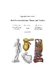
<strong>Spectral</strong> <strong>Mesh</strong> <strong>Processing</strong><br />
SIGGRAPH Asia 2009 Course 32<br />
Bruno Lévy (INRIA, France)<br />
Hao (Richard) Zhang (Simon Fraser University, Canada)
About the instructors<br />
Bruno Lévy<br />
INRIA, centre Nancy Grand Est,<br />
rue du Jardin Botanique,<br />
54500 Vandoeuvre, France<br />
Email: bruno.levy@inria.fr<br />
http://<strong>alice</strong>.loria.fr/index.php/bruno-levy.html<br />
Bruno Lévy is a researcher with INRIA. His main contribution concerns parameterization<br />
of triangulated surfaces (LSCM), and is now used by some 3D<br />
modeling software (including Maya, Silo, Blender, Gocad and Catia). He obtained<br />
his Ph.D in 1999, and was hired by INRIA in 2000. Since 2004, he has<br />
been leading Project ALICE - Geometry and Light, that aims at developping<br />
mathematical tools for next generation geometry processing. He served on the<br />
committee of ACM SPM, IEEE SMI, ACM/EG SGP, IEEE Visualization, Eurographics,<br />
PG, ACM Siggraph, and was program co-chair of ACM SPM in 2007<br />
and 2008, and will be program co-chair of SGP 2010. He was recently awarded<br />
a ”Starting Grant” from the European Research Council (3% acceptance, all<br />
disciplines of science).<br />
Hao (Richard) Zhang<br />
School of Computing Science<br />
Simon Fraser University, Burnaby, Canada V5A 1S6<br />
Email: haoz@cs.sfu.ca<br />
http://www.cs.sfu.ca/˜haoz<br />
Hao (Richard) Zhang is an Associate Professor in the School of Computing<br />
Science at Simon Fraser University, Canada, and he co-directs the Graphics,<br />
Usability, and Visualization (GrUVi) Lab. He received his Ph.D. from the<br />
University of Toronto in 2003 and M. Math. and B. Math. degrees from the<br />
University of Waterloo. His research interests include geometry processing,<br />
shape analysis, and computer graphics. He gave a Eurographics State-of-theart<br />
report on spectral methods for mesh processing and analysis in 2007 and<br />
wrote the first comprehensive survey on this topic. Recently, he has served on<br />
the program committees of Eurographics, ACM/EG SGP, ACM/SIAM GPM,<br />
and IEEE SMI. He was a winner of the Best Paper Award from SGP 2008.
Course description<br />
Summary statement: In this course, you will learn the basics of Fourier<br />
analysis on meshes, how to implement it, and how to use it for filtering, remeshing,<br />
matching, compressing, and segmenting meshes.<br />
Abstract: <strong>Spectral</strong> mesh processing is an idea that was proposed at the beginning<br />
of the 90’s, to port the “signal processing toolbox” to the setting of<br />
3D mesh models. Recent advances in both computer horsepower and numerical<br />
software make it possible to fully implement this vision. In the more classical<br />
context of sound and image processing, Fourier analysis was a corner stone<br />
in the development of a wide spectrum of techniques, such as filtering, compression,<br />
and recognition. In this course, attendees will learn how to transfer<br />
the underlying concepts to the setting of a mesh model, how to implement the<br />
“spectral mesh processing” toolbox and use it for real applications, including<br />
filtering, shape matching, remeshing, segmentation, and parameterization.<br />
Background: Some elements of this course appeared in the “Geometric Modeling<br />
based on Polygon <strong>Mesh</strong>es” course (SIGGRAPH 07, Eurographics 08), the<br />
“<strong>Mesh</strong> Parameterization, Theory and Practice” course (SIGGRAPH 07), and<br />
the “<strong>Mesh</strong> <strong>Processing</strong>” course (invited course, ECCV 08). Based on some feedback<br />
from the attendees, it seems that there is a need for a course focused on the<br />
spectral aspects. Whereas these previous courses just mentioned some applications<br />
of spectral methods, this course details the notions relevant to spectral<br />
mesh processing, from theory to implementation. <strong>Spectral</strong> methods for mesh<br />
processing had been presented as a Eurographics State-of-the-art report in 2007<br />
and a subsequent survey was completed in 2009. Some coverages in the current<br />
notes, in particular those on applications, have been selected from the survey.<br />
However, we start with a more basic setup this time and include updates from<br />
some of the most recent developments in spectral mesh processing.<br />
Intended audience: Researcher in the areas of geometry processing, shape<br />
analysis, and computer graphics, as well as practitioners who want to learn more<br />
about how to implement these new techniques and what are the applications.<br />
Prerequisites: Knowledge about mesh processing, programming, mesh data<br />
structures, basic notions of linear algebra and signal processing.
Course syllabus<br />
• (5 min) Introduction [Lévy]<br />
• (45 min) “What is so spectral?” [Zhang]<br />
Intuition and theory behind spectral methods<br />
Different interpretations and motivating applications<br />
• (55 min) Do your own <strong>Spectral</strong> <strong>Mesh</strong> processing at home [Lévy]<br />
DEC Laplacian, numerics of spectral analysis<br />
Tutorial on implementation with open source software<br />
• (15 min) break<br />
• (50 min) Applications - “What can we do with it ?” 1/2 [Zhang]<br />
Segmentation, shape retrieval, non-rigid matching, symmetry detection,<br />
. . .<br />
• (40 min) Applications - “What can we do with it ?” 2/2 [Lévy]<br />
Quadrangulation, parameterization, . . .<br />
• (15 min) Wrapup, conclusion, Q&A [Zhang and Lévy]
<strong>Spectral</strong> mesh processing involves the use of eigenvalues, eigenvectors, or<br />
eigenspace projections derived from appropriately defined mesh operators to<br />
carry out desired tasks. Early work in this area can be traced back to the<br />
seminal paper by Taubin [Tau95a] in 1995, where spectral analysis of mesh<br />
geometry based on a graph Laplacian allows us to understand the low-pass<br />
filtering approach to mesh smoothing. Over the past fifteen years, the list of<br />
geometry processing applications which utilize the eigenstructures of a variety<br />
of mesh operators in different manners have been growing steadily.<br />
Most spectral methods for mesh processing have a basic framework in common.<br />
First, a matrix representing a discrete linear operator based on the topological<br />
and/or geometric structure of the input mesh is constructed, typically as<br />
a discretization of some continuous operator. This matrix can be seen as incorporating<br />
pairwise relations between mesh elements, adjacent ones or otherwise.<br />
Then an eigendecomposition of the matrix is performed, that is, its eigenvalues<br />
and eigenvectors are computed. Resulting structures from the decomposition<br />
are employed in a problem-specific manner to obtain a solution.<br />
We will look at the various applications of spectral mesh processing towards<br />
the end of the course notes (Section 5), after we provide the intuition, motivation,<br />
and some theory behind the use of the spectral approach. The main<br />
motivation for developing spectral methods for mesh processing is the pursuit<br />
of Fourier analysis in the manifold setting, in particular, for meshes which are<br />
the dominant discrete representations of surfaces in the field of computer graphics.<br />
There are other desirable characteristics of the spectral approach including<br />
effective and information-preserving dimensionality reduction and its ability to<br />
reveal global and intrinsic structures in geometric data [ZvKDar]. These should<br />
become clear as we discuss the applications.<br />
We shall start the course notes with a very gentle introduction in Section 1.<br />
Instead of diving into 3D data immediately, we first look at the more classic case<br />
of processing a 2D shape represented by a contour. The motivating application<br />
is shape smoothing. We reduce the 2D shape processing problem to the study<br />
of 1D functions or signals specifying the shape’s contour, naturally exposing the<br />
problem in a signal-processing framework. Our choice to start the coverage in<br />
the discrete setting is intended to not involve the heavy mathematical formulations<br />
at the start so as to better provide an intuition. We present Laplacian<br />
smoothing and show how spectral processing based on 1D discrete Laplace operators<br />
can perform smoothing as well as compression. The relationship between<br />
this type of spectral processing and the classical Fourier transform is revealed<br />
and a natural extension to the mesh setting is introduced.<br />
Having provided an intuition, we then instill more rigor into our coverage and<br />
more formally present spectral mesh processing as a means to perform Fourier<br />
analysis on meshes. In particular, we deepen our examination on the connection<br />
between the continuous and the discrete settings, focusing on the Laplace<br />
operator and its eigenfunctions. While Section 2 provides some theoretical<br />
background in the continuous setting (eigenfunctions of the Laplace-Beltrami<br />
operator) and establishes connections with other domains (machine learning<br />
and spectral graph theory). Section 3 is concerned with ways to discretize the
Laplace operator. Since spectral mesh processing in practice often necessitates<br />
the computation of eigenstructures of large matrices, Section 4 presents ways to<br />
make that process efficient. Finally, we discuss various applications of spectral<br />
mesh processing in Section 5. For readers who wish to obtain a more thorough<br />
coverage on the topic, we refer to the survey of Zhang et al. [ZvKDar].<br />
1 A gentle introduction<br />
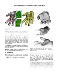
Consider the seahorse shape depicted by a closed contour, shown in Figure 1.<br />
The contour is represented as a sequence of 2D points (the contour vertices) that<br />
are connected by straight line segments (the contour segments), as illustrated<br />
by a zoomed-in view. Now suppose that we wish to remove the rough features<br />
over the shape of the seahorse and obtain a smoothed version, such as the one<br />
shown in the right of Figure 1.<br />
Figure 1: A seahorse with rough features (left) and a smoothed version (right).<br />
1.1 Laplacian smoothing<br />
A simple procedure to accomplish this is to repeatedly connect the midpoints<br />
of successive contour segments; we refer to this as midpoint smoothing. Figures<br />
2(a) illustrates two such steps. As we can see, after two steps of midpoint<br />
smoothing, each contour vertex v i is moved to the midpoint of the line segment<br />
connecting the midpoints of the original contour segments adjacent to v i .<br />
Specifically, let v i−1 = (x i−1 , y i−1 ), v i = (x i , y i ), and v i+1 = (x i+1 , y i+1 ) be<br />
three consecutive contour vertices. Then the new vertex ˆv i after two steps of<br />
midpoint smoothing is given by a local averaging,<br />
ˆv i = 1 [ 1<br />
2 2 (v i−1 + v i )]<br />
+ 1 [ 1<br />
2 2 (v i + v i+1 )]<br />
= 1 4 v i−1 + 1 2 v i + 1 4 v i+1. (1)<br />
The vector between v i and the midpoint of the line segment connecting the<br />
two vertices adjacent to v i , shown as a red arrow in Figure 2(b), is called the
midpoint<br />
smoothing<br />
midpoint<br />
smoothing<br />
(a) Two steps of midpoint smoothing.<br />
v i<br />
Laplacian<br />
smoothing<br />
v i ! 1<br />
v i+1<br />
(b) Laplacian smoothing.<br />
(c) 1D Laplacians (red).<br />
Figure 2: One step of Laplacian smoothing (b) is equivalent to two steps of<br />
midpoint smoothing (a). The 1D discrete Laplacian vectors (c) are in red.<br />
1D discrete Laplacian at v i , denoted by δ(v i ),<br />
δ(v i ) = 1 2 (v i−1 + v i+1 ) − v i . (2)<br />
As we can see, after two steps of midpoint smoothing, each contour vertex is<br />
displaced by half of its 1D discrete Laplacian, as shown in Figure 2(c); this is<br />
referred to as Laplacian smoothing. The smoothed version of the seahorse in<br />
Figure 1 was obtained by applying 10 steps of Laplacian smoothing.<br />
1.2 Signal representation and spectral transform<br />
Let us denote the contour vertices by a coordinate vector V , which has n rows<br />
and two columns, where n is the number of vertices along the contour and the<br />
two columns correspond to the x and y components of the vertex coordinates.<br />
Let us denote by x i (respectively, y i ) the x (respectively, y) coordinate of a vertex<br />
v i , i = 1, . . . , n. For analysis purposes, let us only consider the x component of<br />
V , denoted by X; the treatment of the y component is similar.<br />
We treat the vector X as a discrete 1D signal. Since the contour is closed,<br />
we can view X as a periodic 1D signal defined over uniformly spaced samples<br />
along a circle, as illustrated in Figure 3(a). We sort the contour vertices in<br />
counterclockwise order and plot it as a conventional 1D signal, designating an<br />
arbitrary element in X to start the indexing. Figure 3(b) shows such a plot for<br />
the x-coordinates of the seahorse shape (n = 401) from Figure 1. We can now<br />
express the discrete 1D Laplacians (2) for all the vertices using an n × n matrix
350<br />
X<br />
300<br />
V =<br />
x 1<br />
x 2<br />
......<br />
y1<br />
y 2<br />
......<br />
x i!1<br />
x n<br />
y n<br />
x i<br />
i!1<br />
i<br />
i+1<br />
x<br />
i+1<br />
x−coordinates<br />
250<br />
200<br />
150<br />
0 100 200 300 400<br />
Contour vertex indexes<br />
Figure 3: Left: The x-component of the contour coordinate vector V , X, can<br />
be viewed as a 1D periodic signal defined over uniform samples along a circle.<br />
Right: it is shown by a 1D plot for the seahorse contour from Figure 1.<br />
L, called the 1D discrete Laplace operator, as follows:<br />
⎡<br />
1 − 1 2<br />
0 . . . . . . 0 − 1 ⎤<br />
2<br />
− 1 2<br />
1 − 1 2<br />
0 . . . . . . 0<br />
δ(X) = LX =<br />
⎢ . . . . . . .<br />
X. (3)<br />
⎥<br />
⎣ 0 . . . . . . 0 − 1 2<br />
1 − 1 ⎦<br />
2<br />
− 1 2<br />
0 . . . . . . 0 − 1 2<br />
1<br />
The new contour ˆX resulting from Laplacian smoothing (1) is then given by<br />
⎡<br />
ˆX =<br />
⎢<br />
⎣<br />
ˆx 1<br />
ˆx 2<br />
.<br />
ˆx n−1<br />
ˆx n<br />
⎤ ⎡<br />
⎤ ⎡<br />
1 1<br />
1<br />
2 4<br />
0 . . . . . . 0<br />
4<br />
1 1 1<br />
4 2 4<br />
0 . . . . . . 0<br />
=<br />
⎥ ⎢ . . . . . . .<br />
⎥ ⎢<br />
⎦ ⎣<br />
1 1 1<br />
0 . . . . . . 0 ⎦ ⎣<br />
4 2 4<br />
1<br />
1 1<br />
4<br />
0 . . . . . . 0<br />
4 2<br />
x 1<br />
x 2<br />
.<br />
x n−1<br />
x n<br />
The smoothing operator S is related to the Laplace operator L by<br />
S = I − 1 2 L.<br />
⎤<br />
= SX. (4)<br />
⎥<br />
⎦<br />
To analyze the behavior of Laplacian smoothing, in particular what happens<br />
in the limit, we rely on the set of basis vectors formed by the eigenvectors of<br />
L. This leads to a framework for spectral analysis of geometry. From linear<br />
algebra, we know that since L is symmetric, it has real eigenvalues and a set of<br />
real and orthogonal set of eigenvectors which form a basis. Any vector of size<br />
n can be expressed as a linear sum of these basis vectors. We are particularly<br />
interested in such an expression for the coordinate vector X. Denote by e 1 ,<br />
e 2 ,. . .,e n the normalized eigenvectors of L, corresponding to eigenvalues λ 1 , λ 2 ,<br />
. . ., λ n , and let E be the matrix whose columns are the eigenvectors. Then we
0.1<br />
Eigenvalue ! =0.000000<br />
0.1<br />
Eigenvalue ! =0.000123<br />
0.1<br />
Eigenvalue ! =0.000123<br />
0.1<br />
Eigenvalue ! =0.000491<br />
0.05<br />
0.05<br />
0.05<br />
0.05<br />
0<br />
0<br />
0<br />
0<br />
−0.05<br />
−0.05<br />
−0.05<br />
−0.05<br />
−0.1<br />
100 200 300 400<br />
−0.1<br />
100 200 300 400<br />
−0.1<br />
100 200 300 400<br />
−0.1<br />
100 200 300 400<br />
0.1<br />
Eigenvalue ! =0.000491<br />
0.1<br />
Eigenvalue ! =0.001105<br />
0.1<br />
Eigenvalue ! =0.001105<br />
0.1<br />
Eigenvalue ! =0.001963<br />
0.05<br />
0.05<br />
0.05<br />
0.05<br />
0<br />
0<br />
0<br />
0<br />
−0.05<br />
−0.05<br />
−0.05<br />
−0.05<br />
−0.1<br />
100 200 300 400<br />
−0.1<br />
100 200 300 400<br />
−0.1<br />
100 200 300 400<br />
−0.1<br />
100 200 300 400<br />
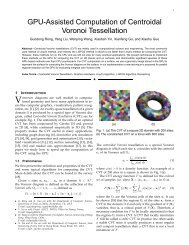
Figure 4: Plots of first 8 eigenvectors of the 1D discrete Laplace operator (n =<br />
401) given in equation (3). They are sorted by the eigenvalue λ.<br />
can express X as a linear sum of the eigenvectors,<br />
⎡ ⎤ ⎡ ⎤ ⎡<br />
⎤ ⎡ ⎤<br />
E 11<br />
E 1n E 11 . . . E 1n ˜x 1<br />
n∑<br />
E 21<br />
X = e i˜x i = ⎢<br />
⎣<br />
⎥<br />
⎦ ˜x E 2n<br />
1 + . . . + ⎢<br />
⎣<br />
⎥<br />
i=1<br />
.<br />
⎦ ˜x E 21 . . . E 2n<br />
˜x 2<br />
n = ⎢<br />
⎣<br />
.<br />
.<br />
⎥ ⎢<br />
.<br />
⎦ ⎣<br />
⎥<br />
.<br />
⎦ = E ˜X.<br />
.<br />
E n1 E nn E n1 . . . E nn ˜x n<br />
(5)<br />
The above expression represents a transform from the original signal X to a<br />
new signal ˜X in terms of a new basis, the basis given by the eigenvectors of L.<br />
We call this a spectral transform, whose coefficients ˜X can be obtained by<br />
˜X = E T X, where E T is the transpose of E,<br />
and for each i, the spectral transform coefficient<br />
˜x i = e T i · X. (6)<br />
That is, the spectral coefficient ˜x i is obtained as a projection of the signal X<br />
along the direction of the i-th eigenvector e i . In Figure 4, we plot the first 8<br />
eigenvectors of L, sorted by increasing eigenvalues, where n = 401, maching<br />
the size of the seahorse shape from Figure 1. The indexing of elements in<br />
each eigenvector follows the same contour vertex indexing as X, the coordinate<br />
vector; it was plotted in Figure 3(b) for the seahorse. It is worth noting that<br />
aside from an agreement on indexing, the Laplace operator L and the eigenbasis<br />
vectors do not depend on X, which specifies the geometry of the contour. L,<br />
as defined in equation (3), is completely determined by n, the size of the input<br />
contour, and a vertex ordering.<br />
As we can see, the eigenvector corresponding to the zero eigenvalue is a<br />
constant vector. As eigenvalue increases, the eigenvectors start to oscillate as<br />
sinusoidal curves at higher and higher frequencies. Note that the eigenvalues of
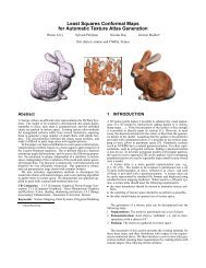
k = 3. k = 5. k = 10. k = 20. k = 30. k ≈ 1 2n. Original.<br />
Figure 5:<br />
Shape reconstruction via Laplacian-based spectral analysis.<br />
L repeat (multiplicity 2) after the first one, hence the corresponding eigenvectors<br />
of these repeated eigenvalues are not unique. One particular choice of the<br />
eigenvectors reveals a connection of our spectral analysis to the classical Fourier<br />
analysis; this will be discussed in Section 1.5.<br />
1.3 Signal reconstruction and compression<br />
With the spectral transform of a coordinate signal defined as in equation (5),<br />
we can now look at compression and filtering of a 2D shape represented by a<br />
contour. Analogous to image compression using JPEG, we can obtain compact<br />
representations of a contour by retaining the leading (low-frequency) spectral<br />
transform coefficients and eliminating the rest. Given a signal X as in equation<br />
(5), the signal reconstructed by using the k leading coefficients is<br />
X (k) =<br />
k∑<br />
e i˜x i , k ≤ n. (7)<br />
i=1<br />
This represents a compression of the contour geometry since only k out of n<br />
coefficients need to be stored to approximate the original shape. We can quantify<br />
the information loss by measuring the L 2 error<br />
n∑<br />
n∑<br />
||X − X (k) || = || e i˜x i || = √ ˜x 2 i ,<br />
i=k+1<br />
i=k+1<br />
which is simply the Euclidean distance between X and X (k) . The last equality<br />
is easy to obtain if we note the orthogonality of the eigenvectors, i.e., e T i ·e j = 0<br />
whenever i ≠ j. Also, since the e i ’s are normalized, e T i · e i = 1.<br />
In Figure 5, we show some results of this type of shape reconstruction (7),<br />
with varying k for the seahorse and a bird shape. As more and more highfrequency<br />
spectral coefficients are removed, i.e., with decreasing k, we obtain
2<br />
2<br />
<strong>Spectral</strong> transform coefficients for X<br />
1.5<br />
1<br />
0.5<br />
0<br />
−0.5<br />
<strong>Spectral</strong> transform coefficients for X<br />
1.5<br />
1<br />
0.5<br />
0<br />
−0.5<br />
−1<br />
0 50 100 150 200 250 300 350 400<br />
Eigenvalue indexes<br />
−1<br />
0 10 20 30 40 50 60 70<br />
Eigenvalue indexes<br />
Figure 6: Plot of spectral transform coefficients for the x component of a<br />
contour. Left: seahorse. Right: bird. The models are shown in Figure 5.<br />
smoother and smoother reconstructed contours. How effectively a 2D shape can<br />
be compressed this way may be visualized by plotting the spectral transform<br />
coefficients, the ˜x i ’s in (6), as done in Figure 6. In the plot, the horizontal<br />
axis represents eigenvalue indexes, i = 1, . . . , n, which roughly correspond to<br />
frequencies. One can view the magnitude of the ˜x i ’s as the energy of the input<br />
signal X at different frequencies.<br />
A signal whose energies are sharply concentrated in the low-frequency end<br />
can be effectively compressed at a high compression rate, since as a consequence,<br />
the total energy at the high-frequency end, representing the reconstruction error,<br />
is very low. Such signals will exhibit fast decay in its spectral coefficients. Both<br />
the seahorse and the bird models contain noisy or sharp features so they are<br />
not as highly compressible as a shape with smoother boundaries. This can be<br />
observed from the plots in Figure 6. Nevertheless, at 2:1 compression ratio, we<br />
can obtain a fairly good approximation, as one can see from Figure 5.<br />
1.4 Filtering and Laplacian smoothing<br />
Compression by truncating the vector ˜X of spectral transform coefficients can<br />
be seen as a filtering process. When a discrete filter function f is applied to ˜X,<br />
we obtain a new coefficient vector ˜X ′ , where ˜X ′ (i) = f(i) · ˜X(i), for all i. The<br />
filtered signal X ′ is then reconstructed from ˜X ′ by X ′ = E ˜X ′ , where E is the<br />
matrix of eigenvectors as defined in equation (5). We next show that Laplacian<br />
smoothing is one particular filtering process. Specifically, when we apply the<br />
Laplacian smoothing operator S to a coordinate vector m times, the resulting<br />
coordinate vector becomes,<br />
X (m) = S m X = (I − 1 2 L)m X =<br />
n∑<br />
(I − 1 2 L)m e i˜x i =<br />
i=1<br />
n∑<br />
e i (1 − 1 2 λ i) m˜x i . (8)<br />
Equation (8) provides a characterization of Laplacian smoothing in the spectral<br />
domain via filtering and the filter function is given by f(λ) = (1 − 1 2 λ)m .<br />
A few such filters with different m are plotted in the first row of Figure 7. The<br />
i=1
1<br />
1<br />
1<br />
1<br />
0.8<br />
0.8<br />
0.8<br />
0.8<br />
0.6<br />
0.6<br />
0.6<br />
0.6<br />
0.4<br />
0.4<br />
0.4<br />
0.4<br />
0.2<br />
0.2<br />
0.2<br />
0.2<br />
0<br />
0 0.5 1 1.5 2<br />
0<br />
0 0.5 1 1.5 2<br />
0<br />
0 0.5 1 1.5 2<br />
0<br />
0 0.5 1 1.5 2<br />
Figure 7: First row: filter plots, (1 − 1 2 λ)m with m = 1, 5, 10, 50. Second row:<br />
corresponding results of Laplacian smoothing on the seahorse.<br />
corresponding Laplacian smoothing leads to attenuation of the high-frequency<br />
content of the signal and hence achieves denoising or smoothing.<br />
To examine the limit behavior of Laplacian smoothing, let us look at equation<br />
(8). Note that it can be shown (via the Gerschgorin’s Theorem [TB97]) that<br />
the eigenvalues of the Laplace operator are in the interval [0, 2] and the smallest<br />
eigenvalue λ 1 = 0. Since λ ∈ [0, 2], the filter function f(λ) = (1 − 1 2 λ)m<br />
is bounded by the unit interval [0, 1] and attains the maximum f(0) = 1 at<br />
λ = 0. As m → ∞, all the terms in the right-hand side of equation (8) will<br />
vanish except for the first, which is given by e 1˜x 1 . Since e 1 , the eigenvector<br />
corresponding to the zero eigenvalue is a normalized, constant vector, we have<br />
e 1 = [ √ 1 √n 1 1<br />
n<br />
. . . √n ] T . Now taking the y-component into consideration, we<br />
1<br />
get the limit point for Laplacian smoothing as √n [˜x 1 ỹ 1 ]. Finally, noting that<br />
˜x 1 = e T 1 · X and ỹ 1 = e T 1 · Y , we conclude that the limit point of Laplacian<br />
smoothing is the centroid of the set of original contour vertices.<br />
1.5 <strong>Spectral</strong> analysis vs. discrete Fourier transform<br />
The sinosoidal behavior of the eigenvectors of the 1D discrete Laplace operator<br />
(see plots in Figure 4) leads one to believe that there must be a connection<br />
between the discrete Fourier transform (DFT) and the spectral transform we<br />
have defined so far. We now make that connection explicit. Typically, one<br />
introduces the DFT in the context of Fourier series expansion. Given a discrete<br />
signal X = [x 1 x 2 . . . x n ] T , its DFT is given by<br />
˜X(k) = 1 n<br />
n∑<br />
X(k)e −i2π(k−1)(j−1)/n , k = 1, . . . , n.<br />
j=1
And the corresponding inverse DFT is given by<br />
or<br />
X =<br />
n∑<br />
k=1<br />
X(j) =<br />
n∑<br />
k=1<br />
˜X(k)e i2π(j−1)(k−1)/n , j = 1, . . . , n,<br />
˜X(k)g k , where g k (j) = e i2π(j−1)(k−1)/n , k = 1, . . . , n.<br />
We see that in the context of DFT, the signal X is expressed as a linear combination<br />
of the complex exponential DFT basis functions, the g k ’s. The coefficients<br />
are given by the ˜X(k)’s, which form the DFT of X. Fourier analysis, provided<br />
by the DFT in the discrete setting, is one of the most important topics in mathematics<br />
and has wide-ranging applications in many scientific and engineering<br />
disciplines. For a systematic study of the subject, we refer the reader to the<br />
classic text by Bracewell [Bra99].<br />
The connection we seek, between DFT and spectral analysis with respect to<br />
the Laplace operator, is that the DFT basis functions, the g k ’s, form a set of<br />
eigenvectors of the 1D discrete Laplace operator L, as defined in (3). A proof of<br />
this fact can be found in Jain’s classic text on image processing [Jai89], where a<br />
stronger claim with respect to circulant matrices was made. Note that a matrix<br />
is circulant if each row can be obtained as a shift (with circular wrap-around)<br />
of the previous row. It is clear that L is circulant.<br />
Specifically, if we sort the eigenvalues of L in ascending order, then they are<br />
λ k = 2 sin 2 π⌊k/2⌋ , k = 2, . . . , n. (9)<br />
n<br />
The first eigenvalue λ 1 is always 0. We can see that every eigenvalue of L, except<br />
for the first, and possibly the last, has a multiplicity of 2. That is, it corresponds<br />
to an eigensubspace spanned by two eigenvectors. If we define the matrix G of<br />
DFT basis as G kj = e i2π(j−1)(k−1)/n , 1 ≤ k, j ≤ n, then the first column of G<br />
is an eigenvector corresponding to λ 1 and the k-th and (n + 2 − k)-th columns<br />
of G are two eigenvectors corresponding to λ k , for k = 2, . . . , n. The set of<br />
eigenvectors of L is not unique. In particular, it has a set of real eigenvectors;<br />
some of these eigenvectors are plotted in Figure 4.<br />
1.6 Towards spectral mesh transform<br />
Based on the above observation, one way to extend the notion of Fourier analysis<br />
to the manifold or surface setting, where our signal will represent the geometry<br />
of the surfaces, is to define appropriate discrete Laplace operators for meshes and<br />
rely on the eigenvectors of the Laplace operators to perform Fourier analysis.<br />
This was already observed in Taubin’s seminal paper [Tau95b].<br />
To extend spectral analysis of 1D signals presented in Section 1.2 to surfaces<br />
modeled by triangle meshes, we first need to extend the signal representation.<br />
This is quite straightforward: any function defined on the mesh vertices can be<br />
seen as a discrete mesh signal. Typically, we focus on the coordinate signal for
(a) Original. (b) k = 300. (c) k = 200. (d) k = 100.<br />
(e) k = 50. (f) k = 10. (g) k = 5. (h) k = 3.<br />
Figure 8: Shape reconstruction based on spectral analysis using a typical mesh<br />
Laplace operator, where k is the number of eigenvectors or spectral coefficients<br />
used. The original model has 7,502 vertices and 15,000 faces.<br />
the mesh, which, for a mesh with n vertices, is an n × 3 matrix whose columns<br />
specify the x, y, and z coordinates of the mesh vertices.<br />
The main task is to define an appropriate Laplace operator for the mesh.<br />
Here a crucial difference to the classical DFTs is that while the DFT basis functions<br />
are fixed as long as the length of the signal in question is determined, the<br />
eigenvectors of a mesh Laplace operator would change with the mesh connectivity<br />
and/or geometry. Formulations for the construction of appropriate mesh<br />
Laplace operators will be the subjects of Sections 2 and 3.<br />
Now with a mesh Laplace operator chosen, defining the spectral transform<br />
of a mesh signal X with respect to the operator is exactly the same as the 1D<br />
case for L in Section 1.2. Denote by e 1 , e 2 ,. . .,e n the normalized eigenvectors of<br />
the mesh Laplace operator, corresponding to eigenvalues λ 1 ≤ λ 2 ≤ . . . ≤ λ n ,<br />
and let E be the matrix whose columns are the eigenvectors. The vector of<br />
spectral transform coefficients ˜X is obtained by ˜X = E T X. And for each i, we<br />
obtain the spectral coefficient by ˜x i = e T i · X via projection.<br />
As a first visual example, we show in Figure 8 some results of spectral reconstruction,<br />
as define in (7), of a mesh model with progressively more spectral<br />
coefficients added. As we can see, higher-frequency contents of the geometric<br />
mesh signal manifest themselves as rough geometric features over the shape’s<br />
surface; these features can be smoothed out by taking only the low-frequence<br />
spectral coefficients in a reconstruction. A tolerance on such loss of geometric<br />
features would lead to a JPEG-like compression of mesh geometry, as first proposed<br />
by Karni and Gotsman [KG00a] in 2000. More applications using spectral<br />
transforms of meshes will be given in Section 5.
2 Fourier analysis for meshes<br />
The previous section introduced the idea of Fourier analysis applied to shapes,<br />
with the example of a closed curve, for which the frequencies (sine waves) are<br />
naturally obtained as the eigenvectors of the 1D discrete Laplacian. We now<br />
study how to formalize the idea presented in the last subsection, i.e. porting<br />
this setting to the case of arbitrary surfaces. Before diving into the heart of<br />
the matter, we recall the definition of the Fourier transform, that is to say<br />
the continuous version of the discrete signal processing framework presented in<br />
Subsections 1.2 and 1.4.<br />
2.1 Fourier analysis<br />
As in Taubin’s article [Tau95b], we start by studying the case of a closed curve,<br />
but staying in the continuous setting. Given a square-integrable periodic function<br />
f : x ∈ [0, 1] ↦→ f(x), or a function f defined on a closed curve parameterized<br />
by normalized arclength, it is well known that f can be expanded into an<br />
infinite series of sines and cosines of increasing frequencies:<br />
f(x) =<br />
∞∑<br />
˜f k H k (x) ;<br />
k=0<br />
⎧<br />
⎨<br />
⎩<br />
H 0 = 1<br />
H 2k+1 = cos(2kπx)<br />
H 2k+2 = sin(2kπx)<br />
where the coefficients ˜f k of the decomposition are given by:<br />
˜f k =< f, H k >=<br />
∫ 1<br />
0<br />
(10)<br />
f(x)H k (x)dx (11)<br />
and where < ., . > denotes the inner product (i.e. the “dot product” for functions<br />
defined on [0, 1]). See [Arv95] or [Lev06] for an introduction to functional<br />
analysis. The ”Circle harmonics” basis H k is orthonormal with respect<br />
to < ., . >: < H k , H k >= 1, < H k , H l >= 0 if k ≠ l.<br />
The set of coefficients ˜f k (Equation 11) is called the Fourier Transform (FT)<br />
of the function f. Given the coefficients ˜f k , the function f can be reconstructed<br />
by applying the inverse Fourier Transform FT −1 (Equation 10). Our goal is<br />
now to explain the generalization of these notions to arbitrary manifolds. To do<br />
so, we can consider the functions H k of the Fourier basis as the eigenfunctions<br />
of −∂ 2 /∂x 2 : the eigenfunctions H 2k+1 (resp. H 2k+2 ) are associated with the<br />
eigenvalues (2kπ) 2 :<br />
− ∂2 H 2k+1 (x)<br />
∂x 2<br />
= (2kπ) 2 cos(2kπx) = (2kπ) 2 H 2k+1 (x)<br />
This construction can be extended to arbitrary manifolds by considering the<br />
generalization of the second derivative to arbitrary manifolds, i.e. the Laplace<br />
operator and its variants, introduced below. Before studying the continuous<br />
theory, we first do a step backward into the discrete setting, in which it is easier
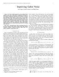
Figure 9: The Fiedler vector gives a natural ordering of the nodes of a graph.<br />
The displayed contours show that it naturally follows the shape of the dragon.<br />
to grasp a geometric meaning of the eigenfunctions. In this setting, eigenfunctions<br />
can be considered as orthogonal non-distorting 1D parameterizations of<br />
the shape, as explained further.<br />
2.2 The discrete setting: Graph Laplacians<br />
<strong>Spectral</strong> graph theory was used for instance in [IL05] to compute an ordering<br />
of vertices in a mesh that facilitates out-of-core processing. Such a natural<br />
ordering can be derived from the Fiedler eigenvector of the Graph Laplacian.<br />
The Graph Laplacian L = (a i,j ) is a matrix defined by:<br />
a i,j = w i,j > 0 if (i, j) is an edge<br />
a i,i = − ∑ j w i,j<br />
a i,j = 0 otherwise<br />
where the coefficients w i,j are weights associated to the edges of the graph. One<br />
may use the uniform weighting w i,j = 1 or more elaborate weightings, computed<br />
from the embedding of the graph. There are several variants of the Graph<br />
Laplacian, the reader is referred to [ZvKDar] for an extensive survey. Among<br />
these discrete Laplacians, the so-called Tutte Laplacian applies a normalization<br />
in each row of L and is given by T = (t i,j ), where<br />
t i,j = P<br />
w i,j<br />
> 0<br />
j<br />
wi,j<br />
if (i, j) is an edge<br />
t i,i = −1<br />
t i,j = 0 otherwise<br />
The Tutte Laplacian was employed in the original work of Taubin [Tau95a],<br />
among others [GGS03a, Kor03].<br />
The first eigenvector of the Graph Laplacian is (1, 1 . . . 1) and its associated<br />
eigenvalue is 0. The second eigenvector is called the Fiedler vector and
has interesting properties, making it a good permutation vector for numerical<br />
computations [Fie73, Fie75]. It has many possible applications, such as finding<br />
natural vertices ordering for streaming meshes [IL05]. Figure 9 shows what it<br />
looks like for a snake-like mesh (it naturally follows the shape of the mesh).<br />
More insight on the Fiedler vector is given by the following alternative definition.<br />
The Fiedler vector u = (u 1 . . . u n ) is the solution of the following constrained<br />
minimization problem:<br />
Minimize: F (u) = u t Lu = ∑ i,j w i,j(u i − u j ) 2<br />
Subject to:<br />
∑<br />
i u i = 0<br />
and<br />
∑<br />
i u2 i = 1 (12)<br />
In other words, given a graph embedded in some space, and supposing that<br />
the edge weight w i,j corresponds to the lengths of the edges in that space, the<br />
Fielder vector (u 1 . . . u n ) defines a (1-dimensional) embedding of the graph on<br />
a line that tries to respect the edge lengths of the graph.<br />
This naturally leads to the question of whether embedding in higher-dimensional<br />
spaces can be computed (for instance, computing a 2-dimensional embedding<br />
of a surface corresponds the the classical surface parameterization problem).<br />
This general problem is well known by the automatic learning research<br />
community as a Manifold learning problem, also called dimension reduction.<br />
One of the problems in manifold learning is extracting from a set of input<br />
(e.g. a set of images of the same object) some meaningful parameters (e.g.<br />
camera orientation and lighting conditions), and sort these images with respect<br />
to these parameters. From an abstract point of view, the images leave in a highdimensional<br />
space (the dimension corresponds to the number of pixels of the<br />
images), and one tries to parameterize this image space. The first step constructs<br />
a graph, by connecting each sample to its nearest neighbors, according to some<br />
distance function. Then, different classes of methods have been defined, we<br />
quickly review the most popular ones:<br />
Local Linear Embedding [RS00a] tries to create an embedding that best<br />
approximates the barycentric coordinates of each vertex relative to its neighbors.<br />
In a certain sense, Floater’s Shape Preserving Parameterization (see [FH04]) is<br />
a particular case of this approach.<br />
Isomap [TdSL00] computes the geodesic distances between each pair of vertex<br />
in the graph, and then uses MDS (multidimensional scaling) [You85] to compute<br />
an embedding that best approximates these distances. Multidimensional<br />
scaling simply minimizes an objective function that measures the deviation between<br />
the geodesic distances in the initial space and the Euclidean distances<br />
in the embedding space (GDD for Geodesic Distance Deviation), by computing<br />
the eigenvectors of the matrix D = (d i,j ) where d i,j denotes the geodesic distance<br />
between vertex i and vertex j. This is a multivariate version of Equation<br />
12, that characterizes the Fiedler vector (in the univariate setting). Isomaps<br />
and Multidimensional scaling were used to define parameterization algorithms<br />
in [ZKK02], and more recently in the ISO-charts method [ZSGS04], used in Microsoft’s<br />
DirectX combined with the packing algorithm presented in [LPM02].
At that point, we understand that the eigenvectors play an important role in<br />
determining meaningful parameters. Just think about the simple linear case: in<br />
PCA (principal component analysis), the eigenvectors of the covariance matrix<br />
characterize the most appropriate hyperplane on which the data should be projected.<br />
In dimension reduction, we seek for eigenvectors that will fit non-linear<br />
features. For instance, in MDS, these eigenvectors are computed in a way that<br />
makes the embedding space mimic the global metric structure of the surface,<br />
captured by the matrix D = (d i,j ) of all geodesic distances between all pairs of<br />
vertices in the graph.<br />
Instead of using the dense matrix D, methods based on the Graph Laplacian<br />
only use local neighborhoods (one-ring neighborhoods). As a consequence, the<br />
used matrix is sparse, and extracting its eigenvectors requires lighter computations.<br />
Note that since the Graph Laplacian is a symmetric matrix, its eigenvectors<br />
are orthogonal, and can be used as a vector basis to represent functions.<br />
This was used in [KG00b] to define a compact encoding of mesh geometry. The<br />
basic idea consists in encoding the topology of the mesh together with the coefficients<br />
that define the geometry projected onto the basis of eigenvectors. The<br />
decoder simply recomputes the basis of eigenvectors and multiplies them with<br />
the coefficients stored in the file. A survey of spectral geometry compression and<br />
its links with graph partitioning is given in [Got03]. <strong>Spectral</strong> graph theory also<br />
enables to exhibit ways of defining valid graph embeddings. For instance, Colinde-verdière’s<br />
number [dV90] was used in [GGS03b] to construct valid spherical<br />
embeddings of genus 0 meshes. Other methods that use spectral graph theory<br />
to compute graph embeddings are reviewed in [Kor02]. <strong>Spectral</strong> graph theory<br />
can also be used to compute topological invariants (e.g. Betti numbers), as<br />
explained in [Fei96]. As can be seen from this short review of spectral graph<br />
theory, the eigenvectors and eigenvalues of the graph Laplacian contain both<br />
geometric and topological information.<br />
However, as explained in [ZSGS04], only using the connectivity of the graph<br />
may lead to highly distorted mappings. Methods based on MDS solve this issue<br />
by considering the matrix D of the geodesic distances between all possible pairs<br />
of vertices. However, we think that it is also possible to inject more geometry<br />
in the Graph Laplacian approach, and understand how the global geometry and<br />
topology of the shape may emerge from the interaction of local neighborhoods.<br />
This typically refers to notions from the continuous setting, i.e. functional<br />
analysis and operators. The next section shows its link with the Laplace-<br />
Beltrami operator, that appears in the wave equation (Helmholtz’s equation).<br />
We will also exhibit the link between the so-called stationary waves and spectral<br />
graph theory.
2.3 The Continuous Setting: Laplace Beltrami<br />
The Laplace operator (or Laplacian) plays a fundamental role in physics and<br />
mathematics. In R n , it is defined as the divergence of the gradient:<br />
∆ = div grad = ∇.∇ = ∑ i<br />
∂x 2 i<br />
∂ 2<br />
Intuitively, the Laplacian generalizes the second order derivative to higher dimensions,<br />
and is a characteristic of the irregularity of a function as ∆f(P )<br />
measures the difference between f(P ) and its average in a small neighborhood<br />
of P .<br />
Generalizing the Laplacian to curved surfaces require complex calculations.<br />
These calculations can be simplified by a mathematical tool named exterior calculus<br />
(EC) 1 . EC is a coordinate free geometric calculus where functions are<br />
considered as abstract mathematical objects on which operators act. To use<br />
these functions, we cannot avoid instantiating them in some coordinate frames.<br />
However, most calculations are simplified thanks to higher-level considerations.<br />
For instance, the divergence and gradient are known to be coordinate free operators,<br />
but are usually defined through coordinates. EC generalizes the gradient<br />
by d and divergence by δ, which are built independently of any coordinate frame.<br />
Using EC, the definition of the Laplacian can be generalized to functions<br />
defined over a manifold S with metric g, and is then called the Laplace-Beltrami<br />
operator:<br />
∆ = div grad = δd = ∑ 1 ∂ √ ∂<br />
√ |g|<br />
i |g| ∂x i ∂x i<br />
where |g| denotes the determinant of g. The additional term √ |g| can be interpreted<br />
as a local ”scale” factor since the local area element dA on S is given by<br />
dA = √ |g|dx 1 ∧ dx 2 .<br />
Finally, for the sake of completeness, we can mention that the Laplacian<br />
can be extended to k-forms and is then called the Laplace-de Rham operator<br />
defined by ∆ = δd + dδ. Note that for functions (i.e. 0-forms), the second term<br />
dδ vanishes and the first term δd corresponds to the previous definition.<br />
Since we aim at constructing a function basis, we need some notions from<br />
functional analysis, quickly reviewed here. A similar review in the context of<br />
light simulation is given in [Arv95].<br />
2.3.1 Functional analysis<br />
In a way similar to what is done for vector spaces, we need to introduce a dot<br />
product (or inner product) to be able to define function bases and project functions<br />
onto those bases. This corresponds to the notion of Hilbert space, outlined<br />
1 To our knowledge, besides Hodge duality used to compute minimal surfaces [PP93],<br />
one of the first uses of EC in geometry processing [GY02] applied some of the fundamental<br />
notions involved in the proof of Poincaré’s conjecture to global conformal parameterization.<br />
More recently, a Siggraph course was given by Schroeder et al. [SGD05], making these notions<br />
usable by a wider community.
elow.<br />
Hilbert spaces<br />
Given a surface S, let X denote the space of real-valued functions defined on<br />
S. Given a norm ‖.‖, the function space X is said to be complete with respect<br />
to the norm if Cauchy sequences converge in X, where a Cauchy sequence is a<br />
sequence of functions f 1 , f 2 , . . . such that lim n,m−>∞ ‖f n −f m ‖ = 0. A complete<br />
vector space is called a Banach space.<br />
The space X is called a Hilbert space in the specific case of the norm defined<br />
by ‖f‖ = √ < f, f >, where < ., . > denotes an inner product. A possible<br />
definition of an inner product is given by < f, g >= ∫ f(x)g(x)dx, which yields<br />
S<br />
the L 2 norm.<br />
One of the interesting features provided by this additional level of structure<br />
is the ability to define function bases and project onto these bases using the<br />
inner product. Using a function basis (Φ i ), a function f will be defined by<br />
f = ∑ α i Φ i . Similarly to the definition in geometry, a function basis (Φ i ) is<br />
orthonormal if ‖Φ i ‖ = 1 for all i and < Φ i , Φ j >= 0 for all i ≠ j. Still following<br />
the analogy with geometry, given the function f, one can easily retrieve its<br />
coordinates α i with respect to an orthonormal basis (Φ i ) by projecting f onto<br />
the basis, i.e. α i =< f, Φ i >.<br />
Operators<br />
We now give the basic definitions related with operators. Simply put, an operator<br />
is a function of functions (i.e. from X to X). An operator L applied<br />
to a function f ∈ X is denoted by Lf, and results in another function in X.<br />
An operator L is said to be linear if L(λf) = λLf for all f ∈ X, λ ∈ R. An<br />
eigenfunction of the operator L is a function f such that Lf = λf. The scalar<br />
λ is an eigenvalue of L. In other words, the effect of applying the operator to<br />
one of its eigenfunctions means simply scaling the function by the scalar λ.<br />
A linear operator L is said to be Hermitian (or with Hermitian symmetry) 2<br />
if < Lf, g >=< f, Lg > for each f, g ∈ X. An important property of Hermitian<br />
operators is that their eigenfunctions associated to different eigenvalues have<br />
real eigenvalues and are orthogonal. This latter property can be easily proven<br />
as follows, by considering two eigenfunctions f, g associated with the different<br />
eigenvalues λ, µ respectively:<br />
< Lf, g > = < f, Lg ><br />
< λf, g > = < f, µg ><br />
λ < f, g > = µ < f, g ><br />
which gives the result (< f, g >= 0) since λ ≠ µ.<br />
As a consequence, considering the eigenfunctions of an Hermitian operator<br />
is a possible way of defining an orthonormal function basis associated to a given<br />
2 the general definition of Hermitian operators concerns complex-valued functions, we only<br />
consider here real-valued functions.
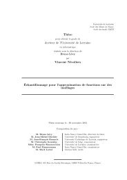
Figure 10: Left: In the late 1700’s, the physicist Ernst Chladni was amazed<br />
by the patterns formed by sand on vibrating metal plates. Right: numerical<br />
simulations obtained with a discretized Laplacian.<br />
function space X. The next section shows this method applied to the Laplace-<br />
Beltrami operator. Before entering the heart of the matter, we will first consider<br />
the historical perspective.<br />
2.3.2 Chladni plates<br />
In 1787, the physicist Ernst Chladni published the book entitled “Discoveries<br />
Concerning the Theories of Music”. In this book, he reports his observations obtained<br />
when putting a thin metal plate into vibration using a bow, and spreading<br />
sand over it. Sand accumulates in certain zones, forming surprisingly complex<br />
patterns (see Figure 10).<br />
This behavior can be explained by the theory of stationary waves. When the<br />
metal plate vibrates, some zones remain still, and sand naturally concentrates in<br />
these zones. This behavior can be modeled as follows, by the spatial component<br />
of Helmholtz’s wave propagation equation:<br />
∆f = λf (13)<br />
In this equation, ∆ denotes the Laplace-Beltrami operator on the considered<br />
object. In Cartesian 2D space, ∆ = ∂ 2 /∂x 2 + ∂ 2 /∂y 2 . We are seeking for the<br />
eigenfunctions of this operator. To better understand the meaning of this equation,<br />
let us first consider a vibrating circle. This corresponds to the univariate<br />
case on the interval [0, 2π] with cyclic boundary conditions (i.e. f(0) = f(2π)).<br />
In this setting, the Laplace-Beltrami operator simply corresponds to the second<br />
order derivative. Recalling that sin(ωx) ′′ = ω 2 sin(ωx), the eigenfunctions are<br />
simply sin(Nx), cos(Nx) and the constant function, where N is an integer. Note<br />
that the so-constructed function basis is the one used in Fourier analysis.<br />
From the spectrum of the Laplace-Beltrami operator, it is well known that<br />
one can extract the area of S, the length of its border and its genus. This<br />
leads to the question asked by Kac in 1966: Can we hear the shape of a drum
Figure 11: Contours of the first eigenfunctions. Note how the protrusions<br />
and symmetries are captured. The eigenfunctions combine the geometric and<br />
topological information contained in the shape signal.<br />
? [Kac66]. The answer to this question is “no”: one can find drums that have<br />
the same spectrum although they do not have the same shape [Cip93] (they are<br />
then referred to as isospectral shapes). However, the spectrum contains much<br />
information, which led to the idea of using it as a signature for shape matching<br />
and classification, as explained in the “shape DNA” approach [RWP05a].<br />
We are now going now to take a look at the eigenfunctions. Mathematicians<br />
mostly studied bounds and convergence of the spectrum. However, some results<br />
are known about the geometry of the eigenfunctions [JNT]. More precisely,<br />
we are interested in the so-called nodal sets, defined to be the zero-set of an<br />
eigenfunction. Intuitively, they correspond to the locations that do not move on<br />
a Chladni plate, where sand accumulates (see Figure 10). A nodal set partitions<br />
the surface into a set of nodal domains of constant sign. The nodal sets and<br />
nodal domains are characterized by the following theorems:<br />
1. the n-th eigenfunction has at most n nodal domains<br />
2. the nodal sets are curves intersecting at constant angles<br />
Besides their orthogonality, these properties make eigenfunction an interesting<br />
choice for function bases. Theorem 1 exhibits their multi-resolution nature,<br />
and from theorem 2, one can suppose that they are strongly linked with the<br />
geometry of the shape. Note also that these theorems explain the appearance<br />
of Chladni plates. This may also explain the very interesting re-meshing results<br />
obtained by Dong et. al [DBG + 05], that use a Morse-smale decomposition of<br />
one of the eigenfunctions.<br />
In the case of simple objects, a closed form of the eigenfunctions can be<br />
derived. This made it possible to retrieve the patterns observed by Chladni in<br />
the case of a square and a circle. For curved geometry, Chladni could not make<br />
the experiment, since sand would not remain in the nodal set. However, one<br />
can still study the eigenfunctions. For instance, on a sphere, the eigenfunction<br />
correspond to spherical harmonics (see e.g. [JNT]), often used in computer<br />
graphics to represent functions defined on the sphere (such as radiance fields or
Figure 12: Contours of the 4th eigenfunction, computed from the Graph Laplacian<br />
(left) and cotangent weights (right) on an irregular mesh.<br />
Bidirectional Reflectance Distribution Functions). In other words, on a sphere,<br />
the eigenfunctions of the Laplace-Beltrami operator define an interesting hierarchical<br />
function basis. One can now wonder whether the same approach could be<br />
used to create function bases on more complex geometries. In the general case,<br />
a closed form cannot be derived, and one needs to use a numerical approach, as<br />
explained in the next section.<br />
3 Discretizing the Laplace operator<br />
The previous section mentioned two different settings for spectral analysis :<br />
• the discrete setting is concerned with graphs, matrices and vectors;<br />
• the continuous setting is concerned with manifolds, operators and functions.<br />
The continuous setting belongs to the realm of differential geometry, a powerful<br />
formalism for studying relations between manifolds and functions defined<br />
over them. However, computer science can only manipulate discrete quantities.<br />
Therefore, a practical implementation of the continuous setting requires a discretization.<br />
This section shows how to convert the continuous setting into a<br />
discrete counterpart using the standard Finite Element Modeling technique. In<br />
Geometry <strong>Processing</strong>, another approach consists in trying to define a discrete<br />
setting that mimics the property of the continous theory. As such, we will also<br />
show how spectral geometry processing can be derived using Discrete Exterior<br />
Calculus (DEC).<br />
The eigenfunctions and eigenvalues of the Laplacian on a (manifold) surface<br />
S, are all the pairs (H k , λ k ) that satisfy:<br />
−∆H k = λ k H k (14)
Figure 13: Some functions of the Manifold Harmonic Basis (MHB) on the Gargoyle<br />
dataset<br />
The “−” sign is here required for the eigenvalues to be positive. On a closed<br />
curve, the eigenfunctions of the Laplace operator define the function basis (sines<br />
and cosines) of Fourier analysis, as recalled in the previous section. On a square,<br />
they correspond to the function basis of the DCT (Discrete Cosine Transform),<br />
used for instance by the JPEG image format. Finally, the eigenfunctions of the<br />
Laplace-Beltrami operator on a sphere define the Spherical Harmonics basis.<br />
In these three simple cases, two reasons make the eigenfunctions a function<br />
basis suitable for spectral analysis of manifolds:<br />
1. Because the Laplacian is symmetric (< ∆f, g >=< f, ∆g >), its eigenfunctions<br />
are orthogonal, so it is extremely simple to project a function<br />
onto this basis, i.e. to apply a Fourier-like transform to the function.<br />
2. For physicists, the eigenproblem (Equation 14) is called the Helmoltz equation,<br />
and its solutions H k are stationary waves. This means that the H k<br />
are functions of constant wavelength (or spatial frequency) ω k = √ λ k .<br />
Hence, using the eigenfunctions of the Laplacian to construct a function basis<br />
on a manifold is a natural way to extend the usual spectral analysis to this<br />
manifold. In our case, the manifold is a mesh, so we need to port this construction<br />
to the discrete setting. The first idea that may come to the mind is to apply<br />
spectral analysis to a discrete Laplacian matrix (e.g. the cotan weights). However,<br />
the discrete Laplacian is not a symmetric matrix (the denominator of the<br />
a i,j coefficient is the area of vertex i ′ s neighborhood, that does not necessarily<br />
correspond to the area of vertex j’s neighborhood). Therefore, we lose the symmetry<br />
of the Laplacian and the orthogonality of its eigenvectors. This makes it<br />
difficult to project functions onto the basis. For this reason, we will clarify the<br />
relations between the continuous setting (with functions and operators), and<br />
the discrete one (with vectors and matrices) in the next section.<br />
In this section, we present two ways of discretizing the Laplace operator on<br />
a mesh. The first approach is based on Finite Element Modeling (FEM) such<br />
as done in [WBH + 07], and converge to the continuous Laplacian under certain<br />
conditions as explained in [HPW06] and [AFW06]. Reuter et al. [RWP05b]<br />
also use FEM to compute the spectrum (i.e. the eigenvalues) of a mesh, which<br />
provides a signature for shape classification. The cotan weights were also used<br />
in [DBG + 06b] to compute an eigenfunction to steer a quad-remeshing process.
The cotan weights alone are still dependent on the sampling as shown in Figure<br />
18-B, so they are usually weighted by the one ring or dual cell area of each<br />
vertex, which makes them loose their symmetry. As a consequence, they are<br />
improper for spectral analysis (18-C). An empirical symmetrization was proposed<br />
in [Lev06] (see Figure 18-D). The FEM formulation enables to preserve<br />
the symmetry property of the continuous counterpart of the Laplace operator.<br />
It is also possible to derive a symmetric Laplacian by using the DEC formulation<br />
(Discrete Exterior Calculus). Then symmetry is recovered by expressing<br />
the operator in a proper basis. This ensures that its eigenfunctions are both geometry<br />
aware and orthogonal (Figure 18-E). Note that a recent important proof<br />
[WMKG07] states that a ”perfect” discrete Laplacian that satisfies all the properties<br />
of the continuous one cannot exist on general meshes. This explains the<br />
large number of definitions for a discrete Laplacian, depending on the desired<br />
properties.<br />
3.1 The FEM Laplacian<br />
In this subsection, we explain the Finite Element Modeling (FEM) formulation<br />
of the discrete Laplacian. The Discrete Exterior Calculus (DEC)formululation,<br />
presented during the course, is described in the next subsection. We have chosen<br />
to include in these course nodes the full derivations for the FEM Laplacian for<br />
the sake of completeness.<br />
To setup the finite element formulation, we first need to define a set of basis<br />
functions used to express the solutions, and a set of test functions onto which<br />
the eigenproblem (Equation 14) will be projected. As it is often done in FEM,<br />
we choose for both basis and test functions the same set Φ i (i = 1 . . . n). We use<br />
the “hat” functions (also called P 1 ), that are piecewise-linear on the triangles,<br />
and that are such that Φ i (i) = 1 and Φ i (j) = 0 if i ≠ j. Geometrically,<br />
Φ i corresponds to the barycentric coordinate associated with vertex i on each<br />
triangle containing i. Solving the finite element formulation of Equation 14<br />
relative to the Φ i ’s means looking for functions of the form: H k = ∑ n<br />
i=1 Hk i Φi<br />
which satisfy Equation 14 in projection on the Φ j ’s:<br />
or in matrix form:<br />
∀j, < −∆H k , Φ j >= λ k < H k , Φ j ><br />
−Qh k = λBh k (15)<br />
where Q i,j =< ∆Φ i , Φ j >, B i,j =< Φ i , Φ j > and where h k denotes the vector<br />
[H k 1 , . . . H k n]. The matrix Q is called the stiffness matrix, and B the mass matrix.<br />
This appendix derives the expressions for the coefficients of the stiffness<br />
matrix Q and the mass matrix B. To do so, we start by parameterizing a triangle<br />
t = (i, j, k) by the barycentric coordinates (or hat functions) Φ i and Φ j of a point<br />
P ∈ t relative to vertices i and j. This allows to write P = k + Φ i e j − Φ j e i<br />
(Figure 14). This yields an area element dA(P ) = e i ∧ e j dΦ i dΦ j = 2|t|dΦ i dΦ j ,
Figure 14: Notations for matrix coefficients computation. Vectors are typed in<br />
bold letters (e i )<br />
where |t| is the area of t, so we get the integral:<br />
∫<br />
∫ 1 ∫ 1−Φi<br />
Φ i Φ j dA = 2|t|<br />
Φ i Φ j dΦ i dΦ j =<br />
|t|<br />
P ∈t<br />
∫ 1<br />
Φ i=0<br />
Φ i=0<br />
Φ j=0<br />
( 1<br />
Φ i (1 − Φ i ) 2 dΦ i = |t|<br />
2 − 2 3 + 1 4)<br />
= |t|<br />
12<br />
which we sum up on the 2 triangles sharing (i, j) to get B i,j = (|t| + |t ′ |/12. We<br />
get the diagonal terms by:<br />
∫<br />
∫ 1 ∫ 1−Φi<br />
Φ 2 i dA = 2|t|<br />
Φ 2 i dΦ j =<br />
P ∈t<br />
Φ i=0<br />
Φ j=0<br />
∫ 1<br />
( 1<br />
2|t| Φ 2 i (1 − Φ i )dΦ i = 2|t|<br />
Φ i=0<br />
3 − 1 4)<br />
= |t|<br />
6<br />
which are summed up over the set St(i) of triangles containing i to get B i,i =<br />
( ∑ t∈St(i) |t|)/6.<br />
To compute the coefficients of the stiffness matrix Q, we use the fact that d<br />
and δ are adjoint to get the more symmetric expression:<br />
∫<br />
Q i,j =< ∆Φ i , Φ j >=< δdΦ i , Φ j >=< dΦ i , dΦ j >= ∇Φ i .∇Φ j<br />
In t, the gradients of barycentric coordinates are the constants :<br />
S<br />
∇Φ i = −e⊥ i<br />
2|t|<br />
∇Φ i .∇Φ j = e i.e j<br />
4|t| 2
Where e ⊥ i denotes e i rotated by π/2 around t’s normal. By integrating on t we<br />
get: ∫<br />
∇Φ i .∇Φ j dA = e i.e j<br />
= ||e i||.||e j || cos(β ij )<br />
4|t| 2||e i ||.||e j || sin(β ij ) = cot(β ij)<br />
2<br />
t<br />
Summing these expressions, the coefficients of the stiffness matrix Q are<br />
given by:<br />
Q i,i =<br />
∑<br />
t∈St(i)<br />
∇Φ i .∇Φ i =<br />
∑<br />
t∈St(i)<br />
e 2 i<br />
4|t|<br />
∫<br />
Q i,j = ∇Φ i .∇Φ j = 1 (<br />
cot(βij ) + cot(β<br />
t∪t 2<br />
ij)<br />
′<br />
′<br />
Note that this expression is equivalent to the numerator of the classical cotan<br />
weights.<br />
{<br />
Qi,j = ( cotan(β i,j ) + cotan(β ′ i,j )) /2<br />
Q i,i = − ∑ j Q i,j<br />
{<br />
Bi,j = (|t| + |t ′ |) /12<br />
B i,i = ( ∑ t∈St(i) |t|)/6 (16)<br />
where t, t ′ are the two triangles that share the edge (i, j), |t| and |t ′ | denote<br />
their areas, β i,j , β i,j ′ denote the two angles opposite to the edge (i, j) in t and<br />
t ′ , and St(i) denotes the set of triangles incident to i.<br />
To simplify the computations, a common practice of FEM consists in replacing<br />
this equation with an approximation:<br />
−Qh k = λDh k (<br />
or − D −1 Qh k = λh k) (17)<br />
where the mass matrix B is replaced with a diagonal matrix D called the lumped<br />
mass matrix, and defined by:<br />
D i,i = ∑ B i,j = ( ∑<br />
|t|)/3. (18)<br />
j<br />
t∈St(i)<br />
Note that D is non-degenerate (as long as mesh triangles have non-zero areas).<br />
FEM researchers [Pra99] explain that besides simplifying the computations this<br />
approximation fortuitously improves the accuracy of the result, due to a cancellation<br />
of errors, as pointed out in [Dye06]. The practical solution mechanism<br />
to solve Equation 17 will be explained further in the section about numerics.<br />
Remark: The matrix D −1 Q in (Equation 17) exactly corresponds to the usual<br />
discrete Laplacian (cotan weights). Hence, in addition to direct derivation of<br />
triangle energies [PP93] or averaged differential values [MDSB03], the discrete<br />
Laplacian can be derived from a lumped-mass FEM formulation.
Figure 15: Reconstructions obtained with an increasing number of eigenfunctions.<br />
As will be seen further, the FEM formulation and associated inner product<br />
will help us understand why the orthogonality of the eigenvectors seems to be<br />
lost (since D −1 Q is not symmetric), and how to retrieve it.<br />
Without entering the details, we mention some interesting features and degrees<br />
of freedom obtained with the FEM formulation. The function basis Φ onto<br />
the eigenfunction problem is projected can be chosen. One can use piecewise<br />
polynomial functions. Figure 16 shows how the eigenfunctions look like with<br />
the usual piecewise linear basis (also called P1 in FEM parlance) and degree 3<br />
polynomial basis (P3). Degree 3 triangles are defined by 10 values (1 value per<br />
vertex, two values per edge and a central value). As can be seen, more complex<br />
function shapes can be obtained (here displayed using a fragment shader). It is<br />
also worth mentioning that the boundaries can be constrained in two different<br />
ways (see Figure 17). With Dirichlet boundary conditions, the value of the function<br />
is constant on the boundary (contour lines are parallel to the boundary).<br />
With Neumann boundary condistions, the gradient of the eigenfunction is parallel<br />
to the boundary (therefore, contour lines are orthogonal to the boundary).<br />
3.2 The DEC Laplacian<br />
For a complete introduction to DEC we refer the reader to [DKT05], [Hir03] and<br />
to [AFW06] for proofs of convergence. We quickly introduce the few notions and<br />
notations that we are using to define the inner product < ., . > and generalized<br />
second-order derivative (i.e. Laplacian operator).<br />
A k-simplex s k is the geometric span of k + 1 points. For instance, 0, 1 and<br />
2-simplices are points, edges and triangles respectively. In our context, a mesh<br />
can be defined as a 2-dimensional simplicial complex S, i.e. a collection of n k<br />
k-simplices (k = 0, 1, 2), with some conditions to make it manifold. A discrete<br />
k-form ω k on S is given by a real value ω k (s k ) associated with each oriented k-<br />
simplex (that corresponds to the integral of a smooth k-form over the simplex).<br />
The set Ω k (S) of k-forms on S is a vector-space of dimension n k . With a proper<br />
numbering of the k-simplices, ω k can be assimilated to a vector of size n k , and<br />
linear operators from Ω k (S) to Ω l (S) can be assimilated to (n k , n l ) matrices.<br />
The exterior derivative d k : Ω k (S) → Ω k+1 (S) is defined by the signed<br />
adjacency matrix: (d k ) sk ,s k+1<br />
= ±1 if s k belongs to the boundary of s k+1 , with<br />
the sign depending on their respective orientations.
Figure 16: Contour lines of eigenfunctions obtained with a linear basis (left)<br />
and a cubic basis (right)<br />
DEC provides Ω k (S) with a L 2 inner product:<br />
< ω k 1 , ω k 2 >= (ω k 1 ) T ⋆ k ω k 2 (19)<br />
where ⋆ k is the so-called Hodge star. As a matrix, the Hodge star is diagonal<br />
with elements |s ∗ k |/|s k| where s ∗ k denotes the circumcentric dual of simplex s k,<br />
and |.| is the simplex volume. In particular, for vertices, edges and triangles:<br />
(⋆ 0 ) vv = |v ∗ | ; (⋆ 1 ) ee = |e∗ |<br />
|e|<br />
= cot β e + cot β ′ e ; (⋆ 2 ) tt = |t| −1<br />
where β e and β ′ e denote the two angles opposite to e.<br />
The codifferential δ k : Ω k (S) → Ω k−1 (S) is the adjoint of the exterior derivative<br />
for the inner product:<br />
< δ k ω k 1 , ω k−1<br />
2 >=< ω k 1 , d k−1 ω k−1<br />
2 ><br />
which yields δ k = − ⋆ −1<br />
k−1 dT k−1 ⋆ k.<br />
Finally the Laplace de Rham operator on k-forms is given by: ∆ k = d k−1 δ k +<br />
δ k+1 d k . In this paper, we are only interested in the Laplacian ∆ = ∆ 0 , i.e. the<br />
Laplace de Rham operator for 0-forms . Since δ 0 and d 2 are undefined (zero by<br />
convention), ∆ = δ 1 d 0 = − ⋆ −1<br />
0 d T 1 ⋆ 1 d 0 and its coefficients are given by:<br />
∆ ij = − cot(β ij) + cot(β ij ′ )<br />
|vi ∗| ; ∆ ii = − ∑ ∆ ij<br />
j<br />
For surfaces with borders, if the edge ij is on the border, the term cot(β ij ′ )<br />
vanishes and the dual cell vi<br />
∗ is cropped by the border. This matches the FEM<br />
formulation with Neumann boundary conditions (not detailed here).
Figure 17: Contour lines of eigenfunctions obtained with Dirichlet boundary<br />
conditions (left) and Neumann boundary conditions (right)
Figure 18: Filtering an irregularly sampled surface (twice denser on the<br />
right half) with different discrete laplacians. Combinatorial Laplacian (A),<br />
unweighted cotan cot(β ij ) + cot(β ij ′ ) (B) and symmetrized weighted cotan<br />
(cot(β ij )+cot(β ij ′ ))/(A i +A j ) (D) produce deformed results (right leg is bigger).<br />
Weighted cotan (cot(β ij )+cot(β ij ′ ))/A i is not symmetric which does not allow for<br />
correct reconstruction (C). Only symmetric weights (cot(β ij )+cot(β ij ′ ))/√ A i A j<br />
is fully mesh-independent (E).<br />
Remark: The matrix ∆ corresponds to the standard discrete Laplacian,<br />
except for the sign. The sign difference comes from the distinction between<br />
Laplace-Beltrami and Laplace de Rham operators.<br />
The so-defined Laplacian ∆ apparently looses the symmetry of its continuous<br />
counterpart (∆ ij ≠ ∆ ji ). This makes the eigenfunction basis no longer<br />
orthonormal, which is problematic for our spectral processing purposes (Figure<br />
18-C). To recover symmetry, consider the canonical basis (φ i ) of 0-forms:<br />
φ i = 1 on vertex i and φ i = 0 on other vertices. This basis is orthogonal<br />
but not normal with respect to the inner product defined in Equation 19<br />
(< φ i , φ i >= (φ i ) T ⋆ 0 φ i ≠ 1). However, since the Hodge star ⋆ 0 is a diagonal<br />
matrix, one can easily normalize (φ i ) as follows:<br />
¯φ i = ⋆ −1/2<br />
0 φ i<br />
In this orthonormalized basis ( ¯φ i ), the Laplacian ¯∆ is symmetric, and its coefficients<br />
are given by:<br />
¯∆ = ⋆ −1/2<br />
0 ∆⋆ 1/2<br />
0 ; ¯∆ij = − cot β ij + cot β ′ ij<br />
√|v ∗ i ||v∗ j | (20)<br />
4 Computing eigenfunctions<br />
Now that we have seen two equivalent discretizations of the Laplacien, namely<br />
FEM (Finite Elements Modeling) and DEC (Discrete Exterior Calculus), we<br />
will now focus on the problem of computing the eigenfunctions in practice. An
implementation of the algorithm is available from the WIKI of the course (see<br />
web reference at the beginning of this document).<br />
Computing the eigenfunctions means solving for the eigenvalues λ k and<br />
eigenvectors ¯H k for the symmetric positive semi-definite matrix ¯∆:<br />
¯∆ ¯H k = λ k ¯Hk<br />
However, eigenvalues and eigenvectors computations are known to be extremely<br />
computationally intensive. To reduce the computation time, Karni et<br />
al. [KG00c] partition the mesh into smaller charts, and [DBG + 06b] use multiresolution<br />
techniques. In our case, we need to compute multiple eigenvectors<br />
(typically a few thousands). This is known to be currently impossible for meshes<br />
with more than a few thousand vertices [WK05]. In this section, we show how<br />
this limit can be overcome by several orders of magnitude.<br />
To compute the solutions of a large sparse eigenproblems, several iterative<br />
algorithms exist. The publicly available library ARPACK (used in [DBG + 06b])<br />
provides an efficient implementation of the Arnoldi method. Yet, two characteristics<br />
of eigenproblem solvers hinder us from using them directly to compute<br />
the MHB for surfaces with more than a few thousand vertices:<br />
• first of all, we are interested in the lower frequencies, i.e. eigenvectors with<br />
associated eigenvalues lower than ωm.<br />
2 Unfortunately, iterative solvers<br />
performs much better for the other end of the spectrum. This can be<br />
explained in terms of filtering as lower frequencies correspond to higher<br />
powers of the smoothing kernel, which may have a poor condition number;<br />
• secondly, we need to compute a large number of eigenvectors (typically<br />
a thousand), and it is well known that computation time is superlinear<br />
in the number of requested eigenpairs. In addition, if the surface is large<br />
(millions of vertices), the MHB does not fit in system RAM.<br />
4.1 Band-by-band computation of the MHB<br />
We address both issues by applying spectral transforms to the eigenproblem.<br />
To get the eigenvectors of a spectral band centered around a value λ S , we start<br />
by shifting the spectrum by λ S , by replacing ¯∆ with ¯∆ − λ S Id. Then, we can<br />
swap the spectrum by inverting this matrix in ∆ SI = ( ¯∆ − λ S Id) −1 . This is<br />
called the Shift-Invert spectral transform, and the new eigenproblem to solve is<br />
given by:<br />
∆ SI ¯Hk = µ k ¯Hk<br />
It is easy to check that ¯∆ and ∆ SI have the same eigenvectors, and that their<br />
eigenvalues are related by λ k = λ S + 1/µ k . Applying an iterative solver to ∆ SI<br />
will return the high end of the spectrum (largest µ’s), corresponding to a band<br />
of eigenvalues of ¯∆ centered around λ S . It is then possible to split the MHB<br />
computation into multiple bands, and obtain a computation time that is linear<br />
in the number of computed eigenpairs. In addition, if the MHB does not fit in
RAM, each band can be streamed into a file. This gives the following algorithm:<br />
(1) λ S ← 0 ; λ last ← 0<br />
(2) while(λ last < ωm)<br />
2<br />
(3) compute an inverse ∆ SI of ( ¯∆ − λ SId)<br />
(4) find the 50 first eigenpairs ( ¯H k , µ k ) of ∆ SI<br />
(5) for k = 1 to 50<br />
(6) λ k ← λ S + 1/µ k<br />
(7) if (λ k > λ last ) write( ¯H k , λ k )<br />
(8) end //for<br />
(9) λ S ← max(λ k ) + 0.4(max(λ k ) − min(λ k ))<br />
(10) λ last ← max(λ k )<br />
(11) end //while<br />
Before calling the eigen solver, we pre-compute ∆ SI with a sparse direct<br />
solver (Line 3). Note that ¯∆ − λ S Id may be singular. This is not a problem<br />
since the spectral transform still works with an indefinite factorization. The<br />
factorized ¯∆ − λ S Id is used in the inner loop of the eigen solver (Line 4). To<br />
factorize ¯∆−λ S Id, we used sparse direct solvers (TAUCS, SUPERLU). For large<br />
models (millions of vertices), we used the sparse OOC (out-of-core) symmetric<br />
indefinite factorization [MIT06] implemented in the future release of TAUCS,<br />
kindly provided by S. Toledo. We then recover the λ’s from the µ’s (Line 6)<br />
and stream-write the new eigenpairs into a file (Line 7). Since the eigenvalues<br />
are centered around the shift λ S , the shift for the next band is given by the last<br />
computed eigenvalue plus slightly less than half the bandwidth to ensure that<br />
the bands overlap and that we are not missing any eigenvalue (Line 9). If the<br />
bands do not overlap, we recompute a larger band until they do.<br />
Note that this is different from the shift-invert spectral transform implemented<br />
by ARPACK, dedicated to iterative solvers. Ours makes use of the<br />
factorization of the matrix, resulting in much better performances.<br />
5 Applications<br />
The eigendecomposition of a discrete mesh Laplace operator provides a set of<br />
eigenvalues and eigenvectors, which can be directly used by an application to<br />
accomplish different tasks. Moreover, the eigenvectors can also be used as a<br />
basis onto which a signal defined on a triangle mesh is projected. The resulting<br />
spectral transform coefficients can be further analyzed or manipulated. Here we<br />
discuss a subset of the applications which utilize the spectral transform or the<br />
eigenvectors of mesh Laplace or more general linear mesh operators.<br />
5.1 Use of eigenvectors<br />
Eigenvectors are typically used to obtain an embedding of the input shape<br />
in the spectral domain, which we call a spectral embedding. After obtaining<br />
the eigendecomposition of a specific operator, the coordinates of vertex
Figure 19: Compared parameterization results obtained with LSCM (left), spectral<br />
parameterization (center) and ABF++ (right).<br />
i in a k-dimensional spectral embedding are given by the i-th row of matrix<br />
V k = [v 1 , . . . , v k ], where v 1 , . . . , v k are the first k eigenvectors from the spectrum<br />
(possibly after scaling). Whether the eigenvectors should be in ascending<br />
or descending order of eigenvalues depends on the operator that is being used.<br />
The choice of k also varies between applications. For planar mesh parameterization,<br />
k is typically 2, while in other applications, a single eigenvector possessing<br />
desirable properties may be selected for a task.<br />
In computer vision and machine learning, spectral methods usually employ a<br />
different operator, the so-called affinity matrix [SM00, Wei99]. Each entry W ij<br />
of an affinity matrix W represents a numerical relation, the affinity, between<br />
two data points i and j, e.g., pixels in an image, vertices in a mesh, or two<br />
face models in the context of face recognition. Note that the affinity matrix<br />
differs from the Laplacian in that affinities between all data pairs are defined.<br />
Therefore this matrix is not sparse in general. In practice, this non-sparse<br />
structure implies more memory requirements and more expensive computations.<br />
The use of affinity matrices for spectral mesh processing has received wide appeal<br />
in computer graphics as well, e.g., for mesh segmentation.<br />
5.1.1 Parameterization and remeshing<br />
In the context of mesh parameterization, spectral methods have the interesting<br />
property of connecting local entities in a way that lets a global behavior<br />
emerge. This property can be used to compute a good base complex [DBG + 06a],<br />
[HZM + 08], or to directly define a parameterization [ZSGS04], [MTAD08], as explained<br />
below. Figure 19 shows that Mullen et.al’s spectral parameterization<br />
achieves a result comparable to ABF++. The interesting point is that it uses a<br />
simple and elegant formulation of the problem (just compute the Fiedler vector
Figure 20: <strong>Spectral</strong> Surface Quadrangulation first computes a Laplace eigenfunction<br />
(A), then extracts its Morse complex (B), smoothes it (C) and uses it<br />
to partition the mesh into quads, that can be parameterized (D).<br />
of the LSCM matrix).<br />
Besides corresponding to a “Fourier basis on meshes”, eigenfunctions can be<br />
used to define parameterizations. For instance, in the context of data analysis,<br />
LLE (Local Linear Embedding) [RS00b] computes an embedding of a graph<br />
that preserves metric relations in local neighborhoods. Similarly, the MDS<br />
method (multidimensional scaling) [You85] computes an embedding that best<br />
approximates all the geodesic distances between the vertices of a graph. Multidimensional<br />
scaling simply minimizes an objective function that measures the<br />
deviation between the geodesic distances in the initial space and the Euclidean<br />
distances in the embedding space (GDD for Geodesic Distance Deviation), by<br />
computing the eigenvectors of the matrix D = (d i,j ) where d i,j denotes the<br />
geodesic distance between vertex i and vertex j. Isomaps and Multidimensional<br />
scaling were used to define parameterization algorithms in [ZKK02], and more<br />
recently in the ISO-charts method [ZSGS04]. <strong>Spectral</strong> analysis also has the<br />
interesting property of defining an orthogonal basis. This property can be used<br />
to avoid the degenerate configurations encountered by linear conformal parameterization<br />
methods [LPRM02], [DMA02]. Those linear methods use “vertex<br />
pinning” to avoid the trivial constant solution, whereas the spectral method<br />
introduced in [MTAD08] computes the first solution orthogonal to the trivial<br />
one, that is to say, the eigenvector associated with the first non-zero eigenvalue.<br />
However, the spectral parameterization methods listed above still need to<br />
partition the mesh into charts. More recently, Dong et al. used the Laplacian to<br />
decompose a mesh into quadrilaterals [DBG + 05, DBG + 06a], in a way that facilitates<br />
constructing a globally smooth parameterization. As shown in Figure 20,<br />
their method first computes one eigenfunction of the Laplacian (the 38 th in this<br />
example), then extract the Morse complex of this function, filters and smoothes<br />
the Morse complex, and uses it to partition the mesh into quads. These quads<br />
are parameterized, and inter-chart smoothness can be further optimized using<br />
global relaxation [KLS03, THCM04]. More recently, a generalization was<br />
proposed [HZM + 08], still based on Laplacian eigenfunctions, and steered by a
guidance vector field.<br />
5.1.2 Clustering and segmentation<br />
One of the most well-known techniques in this regard is spectral clustering [BN03,<br />
KVV00, NJW02]. Interested readers should refer to the recent survey by von<br />
Luxburg [vL06] and the comparative study by Verma and Meilă [VM03]. Ng et<br />
al. [NJW02] presented a clustering method where the entries of the first k eigenvectors<br />
corresponding to the largest eigenvalues of an affinity matrix are used<br />
to obtain the transformed coordinates of the input data points. Additionally,<br />
the embedded points are projected onto the unit k-sphere. Points that possess<br />
high affinities tend to be grouped together in the spectral domain, where a simple<br />
clustering algorithm, such as k-means, can reveal the final clusters. Other<br />
approaches differ only slightly from the core solution paradigm, e.g., in terms<br />
of the operator used and the dimensionality of the embedding.<br />
The ubiquity of the clustering problem makes spectral clustering an extremely<br />
useful technique. Kolluri et al. [KSO04] used spectral clustering to<br />
determine the inside and outside tetrahedra in the context of a Delaunay-based<br />
surface reconstruction algorithm. Liu and Zhang [LZ04] performed mesh segmentation<br />
via spectral clustering. Basically, an affinity matrix is constructed<br />
where the affinity measure depends on both geodesic distances and curvature<br />
information. Next, the eigenvectors given by the eigendecomposition of this<br />
matrix guide a clustering method, which provides patches of faces that define<br />
the different segments of the mesh returned by the segmentation algorithm. It<br />
is shown by example that it can be advantageous to perform segmentation in<br />
the spectral domain, e.g., in terms of higher-quality cut boundaries.<br />
In a follow-up work, Zhang and Liu [ZL05] presented a mesh segmentation<br />
approach based on a recursive 2-way spectral clustering method. Only the first<br />
two largest eigenvectors of the affinity matrix are computed. This provides a<br />
one-dimensional embedding of mesh faces given by the quotient of the entries of<br />
the two eigenvectors. The most salient cut in this embedding is located, given<br />
by a part salience measure [HS97]. The cut provides a segmentation of the<br />
faces into two parts. This process is recursively repeated in order to obtain a<br />
hierarchical binary partitioning of the input mesh.<br />
In yet another follow-up work, Liu and Zhang [LZ07] proposed an algorithm<br />
for mesh segmentation via recursive bisection where at each step, a sub-mesh<br />
embedded in 3D is spectrally projected to 2D and then a contour is extracted<br />
from the planar embedding. Two operators are used in combination to compute<br />
the projection: the well-known graph Laplacian and a geometric operator<br />
designed to emphasize concavity. The two embeddings reveal distinctive shape<br />
semantics of the 3D model and complement each other in capturing the structural<br />
or geometrical aspects of a segmentation. Transforming the shape analysis<br />
problem to the 2D domain also facilitates segmentability analysis and sampling,<br />
where the latter is needed to identify two samples residing on different parts of<br />
the sub-mesh. These two samples are used by the Nyström method in the construction<br />
of a 1D face sequence for finding an optimal cut, as in [ZL05]. Similar
to the technique presented in Section 4, the Nyström method is designed to efficiently<br />
compute eigenvectors of large matrices. However, it relies on sampling<br />
and extrapolation and only approximates the eigenvectors.<br />
Recently, de Goes et al. [dGGV08] presented a hierarchical segmentation<br />
method for articulated bodies. Their approach relies on the diffusion distance,<br />
which is a multi-scale metric based on the heat kernel and computed from the<br />
eigenvectors of the Laplace-Beltrami operator. The diffusion distance is used<br />
to compute a bijection between medial structures and segments of the model.<br />
The medial structures yield a means to further refine the segmentation in an<br />
iterative manner and provide a full hierarchy of segments for the shape.<br />
Huang et al. [HWAG09] also performed hierarchical shape decomposition via<br />
spectral analysis. However, the operator they use encapsulates shape geometry<br />
beyond the static setting. The idea is to define a certain deformation energy and<br />
use the eigenvectors of the Hessian of the deformation energy to characterize the<br />
space of possible deformations of a given shape. The eigenmodes corresponding<br />
to the low-end of the spectrum of the Hessian capture low-energy or in their formulation,<br />
more rigid deformations, called “typical” deformations. The optimal<br />
shape decomposition they compute is one whose optimal articulated (piecewise<br />
rigid) deformation defined on the parts of the decomposition best conforms to<br />
the basis vectors of the space of typical deformations. As a result, their method<br />
tends to identify parts of a shape which would likely remain rigid during the<br />
“typical” deformations.<br />
5.1.3 Shape correspondence and retrieval<br />
Depending on the requirement of the problem at hand, the mesh operator we<br />
use to compute a spectral embedding can be made to incorporate any intrinsic<br />
measure on a shape in order to obtain useful invariance properties, e.g., with<br />
respect to part articulation or bending. In Figure 21, we show 3D spectral<br />
embeddings of a few human and hand models obtained from an operator derived<br />
from geodesic distances over the mesh surfaces. As geodesic distance is bendingtolerant,<br />
the resulting embeddings are normalized with respect to bending and<br />
can facilitate shape retrieval under part articulation [EK03, JZ07].<br />
Elad and Kimmel [EK03] used MDS to compute bending-invariant signatures<br />
for meshes. Geodesic distances between mesh vertices are computed by<br />
fast marching. The resulting spectral embedding effectively normalizes the mesh<br />
shapes with respect to translation, rotation, as well as bending transformations.<br />
The similarity between two shapes is then given by the Euclidean distance between<br />
the moments of the first few eigenvectors, usually less than 15, and these<br />
similarity distances can be used for shape classification.<br />
Inspired by works in computer vision on spectral point correspondence [SB92],<br />
Jain and Zhang [JZvK07] relied on higher-dimensional embeddings based on<br />
the eigenvectors of an affinity matrix to obtain point correspondence between<br />
two mesh shapes. The first k eigenvectors of the affinity matrix encoding the<br />
geodesic distances between pairs of vertices are used to embed the model in a<br />
k-dimensional space; typically k = 5 or 6. After this process is performed for
Figure 21: <strong>Spectral</strong> embeddings (bottom row) of some articulated 3D shapes<br />
(top row). Since the mesh operator is constructed from geodesic distances, the<br />
embeddings are normalized with respect to shape bending.<br />
Figure 22: Eigenvector plots for two similar shapes, both with 252 vertices.<br />
The entries in an eigenvector are color-mapped. As we can see, there is an<br />
“eigenvector switching” occurring between the fifth and sixth eigenvectors. Such<br />
“switching” is difficult to detect from the magnitude of the eigenvalues. The<br />
first 8 eigenvalues for the two shapes are [205.6, 11.4, 4.7, 3.8, 1.8, 0.4, 0.26, 0.1]<br />
and [201.9, 10.9, 6.3, 3.4, 1.8, 1.2, 0.31, 0.25], respectively.<br />
two models, the two embeddings are non-rigidly aligned via thin-plate splines<br />
and the correspondence between the two shapes is given by the proximity of the<br />
vertices after such alignment. Any measure for the cost of a correspondence,<br />
e.g., sum of distances between corresponding vertices, can be used as a similarity<br />
distance for shape retrieval.<br />
One of the key observations made in [JZvK07] is the presence of “eigenvector<br />
switching” due to non-uniform scaling of the shapes. Specifically, the<br />
eigenmodes of similar shapes do not line up with respect to the magnitude of<br />
their corresponding eigenvalues, as illustrated in Figure 22. As a result, it is<br />
unreliable to sort the eigenvectors according to the magnitude of their respective<br />
eigenvalues, as has been done in all works on spectral correspondence so far.<br />
Jain and Zhang [JZvK07] relied on a heuristic to “unswitch” the eigenmodes and<br />
thin-plate splines to further align the shapes in the spectral domain [JZvK07].<br />
Recent work of Mateus et al. [MCBH07] addressed the issue using an alignment<br />
by the Expectation-Maximization (EM) algorithm instead.<br />
The method by Leordeanu and Hebert [LH05] focuses on the global characteristics<br />
of correspondence computation and aims at finding consistent cor-
espondences between two sets of shape or image features, where the spectral<br />
approach has also found its utility. They build a graph whose nodes represent<br />
possible feature pairings and edge weights measure how agreeable the pairings<br />
are. The principal eigenvector of an affinity matrix W , one corresponding to the<br />
largest eigenvalue, is inspected to detect how strongly the graph nodes belong<br />
to the main cluster of W . The idea is that correct correspondences are likely to<br />
establish links among each other and thus form a strongly connected cluster.<br />
To define informative shape descriptors, another possibility consists in using<br />
the heat diffusion equation and the heat kernel. Heat diffusion is governed by<br />
the following differential equation :<br />
∂f<br />
∂t = k∆f<br />
where k is a constant. This equation admits a solution that can be written as :<br />
∫<br />
f(t, x) = K(t, y, x)dy<br />
where K(t, x, y) denotes the heat kernel. Intuitively, considering that a Dirac of<br />
heat was emitted from point x at time t = 0, the heat kernel K(t, x, y) indicates<br />
the quantity of heat that can be measured at point y after time t. The heat<br />
kernel admits an expression as an (infinite) sum of eigenfunctions :<br />
K(t, x, y) =<br />
∞∑<br />
e −λit φ i (x)φ i (y)<br />
i=0<br />
Using this expression, the idea of using the auto-diffusion function was simultaneously<br />
proposed in [SOG] and [GBAL]. The auto-diffusion function corresponds<br />
to the amount of heat that remains at point x after time t for a given<br />
t, in other words K(t, x, x). This defines a scalar field on the surface that provably<br />
has good properties to be used as a shape descriptor [SOG]. In particular,<br />
protrusions correspond to extrema of the function. The value of t acts as a<br />
smoothing parameter (smaller values of t preserve most details, and higher values<br />
of t tend to a constant function). Another application of the auto-diffusion<br />
function is to compute a Morse-Smale complex for shape segmentation [GBAL].<br />
5.1.4 Global intrinsic symmetry detection<br />
Ovsjanikov et al. [OSG08] propose an approach to detect the intrinsic symmetries<br />
of a shape which are invariant to isometry preserving transformations.<br />
They show that if the shape is embedded into a signature space defined by the<br />
eigenfunctions of the Laplace-Beltrami operator, then the intrinsic symmetries<br />
are transformed into extrinsic Euclidean symmetries (rotations or reflections).<br />
However, it is possible to restrict the search of symmetries only to reflections,<br />
avoiding the search for rotational symmetries, a task that can be hard in highdimensional<br />
space. This result allows to obtain the intrinsic symmetries by<br />
first computing the eigenvectors of the operator, then embedding the shape into
the signature space, and finally finding point-to-point correspondences between<br />
symmetric points. The signature adopted is derived from the GPS embedding<br />
of Rustamov [Rus07].<br />
5.2 Use of spectral transforms<br />
The spectral mesh transforms are closely related to the Fourier transform that<br />
is the foundation of signal processing theory. Conceivably, any application of<br />
the classical Fourier transform in signal or image processing has the potential<br />
to be realized in the mesh setting. In geometry processing, the mesh signal<br />
considered is often the embedding function that specifies the 3D coordinates of<br />
each vertex. This signal serves to represent mesh geometry.<br />
5.2.1 Geometry compression<br />
Karni and Gotsman [KG00c] proposed an approach to compress the geometry<br />
of triangle meshes. Firstly, the set of eigenvectors of the Tutte Laplacian is<br />
computed. Next, the mesh vertex coordinates are projected into the spectral<br />
space spanned by the computed eigenvectors. Part of the coefficients obtained by<br />
this transformation is eliminated in order to reduce the storage space required<br />
for mesh geometry. The coefficients related to the eigenvectors associated to<br />
larger eigenvalues are firstly removed, which would correspond to high frequency<br />
detail, when following an analogy with Fourier analysis.<br />
The main drawback of this method is that many eigenvectors need to be<br />
computed. Karni and Gotsman propose to partition the mesh into smaller sets of<br />
vertices. Although that alleviates the problem of computing the eigenvectors for<br />
large matrices, it still requires a good partitioning of the mesh for the efficiency<br />
of the compression, and artifacts along the partition boundaries are evident<br />
when higher compression rates are employed.<br />
5.2.2 Watermarking<br />
Ohbuchi et al. [OTMM01, OMT02] also employed the spectral transform approach,<br />
but to insert watermarks into triangle meshes. In their method, the<br />
eigenvectors of the graph Laplacian are used as the basis for the projection.<br />
After transforming the geometry of the mesh and obtaining the spectral coefficients,<br />
a watermark is inserted into the model by modifying coefficients at the<br />
low-frequency end of the spectrum. In this way, modifications on the geometry<br />
of the mesh are well-spread over the model and less noticeable than if they were<br />
directly added to the vertex coordinates. This method also requires the computation<br />
of eigenvectors of the Laplace operator, which is prohibitive in the case<br />
of large meshes. <strong>Mesh</strong> partitioning is again used to address this problem.<br />
5.2.3 Fourier descriptors<br />
2D Fourier descriptors have been quite successful as a means to characterize<br />
2D shapes. Using eigendecomposition with respect to the mesh Laplacians,
one can compute analogous Fourier-like descriptors to describe mesh geometry.<br />
However, there have not seen such mesh Fourier descriptors being proposed for<br />
shape analysis so far. There have been methods, e.g., [VS01], which rely on<br />
3D Fourier descriptors for 3D shape retrieval. In this case, the mesh shapes<br />
are first voxelized and 3D Fourier descriptors are extracted from the resulting<br />
volumetric data. We suspect that the main difficulties with the use of mesh<br />
Fourier descriptors for shape matching include computational costs and the fact<br />
that when the eigenmodes vary between the two mesh shapes to be matched,<br />
it becomes doubtful whether their associated eigenspace projections can serve<br />
as reliable shape descriptors. Also, even when the shapes are very similar,<br />
eigenvector switching, as depicted in Figure 22, can occur when the eigenvectors<br />
are ordered by the magnitude of their eigenvalues.<br />
References<br />
[AFW06]<br />
[Arv95]<br />
D. N. Arnold, R. S. Falk, and R. Winther. Finite element exterior<br />
calculus, homological techniques, and applications. Acta Numerica<br />
15, 2006.<br />
James Arvo. The Role of Functional Analysis in Global Illumination.<br />
In P. M. Hanrahan and W. Purgathofer, editors, Rendering<br />
Techniques ’95 (Proceedings of the Sixth Eurographics Workshop on<br />
Rendering), pages 115–126, New York, NY, 1995. Springer-Verlag.<br />
[BN03] M. Belkin and P. Niyogi. Laplacian eigenmaps and spectral<br />
techniques for embedding and clustering. Neural Computations,<br />
15(6):1373–1396, 2003.<br />
[Bra99]<br />
[Cip93]<br />
[DBG + 05]<br />
Ronald N. Bracewell. The Fourier Transform And Its Applications.<br />
McGraw-Hill, 1999.<br />
Barri Cipra. You can’t always hear the shape of a drum. What’s<br />
Happening in the Mathematical Sciences, 1, 1993.<br />
S. Dong, P.-T. Bremer, M. Garland, V. Pascucci, and J. C. Hart.<br />
Quadrangulating a mesh using laplacian eigenvectors. Technical<br />
report, June 2005.<br />
[DBG + 06a] S. Dong, P.-T. Bremer, M. Garland, V. Pascucci, and J. C. Hart.<br />
<strong>Spectral</strong> mesh quadrangulation. ACM Transactions on Graphics<br />
(SIGGRAPH 2006 special issue), 2006.<br />
[DBG + 06b] Shen Dong, Peer-Timo Bremer, Michael Garland, Valerio Pascucci,<br />
and John C. Hart. <strong>Spectral</strong> surface quadrangulation. In SIG-<br />
GRAPH ’06: ACM SIGGRAPH 2006 Papers, pages 1057–1066,<br />
New York, NY, USA, 2006. ACM Press.
[dGGV08]<br />
[DKT05]<br />
Fernando de Goes, Siome Goldenstein, and Luiz Velho. A hierarchical<br />
segmentation of articulated bodies. Computer Graphics Forum<br />
(Symposium on Geometry <strong>Processing</strong>), 27(5):1349–1356, 2008.<br />
Mathieu Desbrun, Eva Kanzo, and Yiying Tong. Discrete differential<br />
forms for computational modeling. Siggraph ’05 course notes<br />
on Discrete Differential Geometry, Chapter 7, 2005.<br />
[DMA02] Mathieu Desbrun, Mark Meyer, and Pierre Alliez. Intrinsic parameterizations<br />
of surface meshes. In Proceedings of Eurographics,<br />
pages 209–218, 2002.<br />
[dV90]<br />
[Dye06]<br />
[EK03]<br />
[Fei96]<br />
[FH04]<br />
[Fie73]<br />
[Fie75]<br />
[GBAL]<br />
Y. Colin de Verdiere. Sur un nouvel invariant des graphes et un<br />
critere de planarite. J. of Combinatorial Theory, 50, 1990.<br />
Ramsey Dyer. Mass weights and the cot operator (personal communication).<br />
Technical report, Simon Fraser University, CA, 2006.<br />
A. Elad and R. Kimmel. On bending invariant signatures for surfaces.<br />
IEEE Trans. Pattern Anal. Mach. Intell., 25(10):1285–1295,<br />
2003.<br />
J. Feidman. Computing betti numbers via combinatorial laplacians.<br />
In Proc. 28th Sympos. Theory Comput., pages 386–391. ACM, 1996.<br />
M. S. Floater and K. Hormann. Surface parameterization: a tutorial<br />
and survey. Springer, 2004.<br />
Miroslav Fiedler. Algebraic connectivity of graphs. Czech. Math.<br />
Journal, 23:298–305, 1973.<br />
Miroslav Fiedler. A property of eigenvectors of nonnegative symmetric<br />
matrices and its application to graph theory. Czech. Math.<br />
Journal, 25:619–633, 1975.<br />
Katarzyna Gebal, Andreas Baerentzen, Henrik Aanaes, and Rasmus<br />
Larsen. Shape analysis using the auto diffusion function. Computer<br />
Graphics Forum (Proc. of Symp. on Geom. Proc.).<br />
[GGS03a] C. Gotsman, X. Gu, and A. Sheffer. Fundamentals of spherical<br />
parameterization for 3d meshes. ACM Trans. Graph., 22(3):358–<br />
363, 2003.<br />
[GGS03b] C. Gotsman, X. Gu, and A. Sheffer. Fundamentals of spherical<br />
parameterization for 3d meshes, 2003.<br />
[Got03]<br />
Craig Gotsman. On graph partitioning, spectral analysis, and digital<br />
mesh processing. In Shape Modeling International, pages 165–<br />
174, 2003.
[GY02]<br />
X. Gu and S.-T. Yau. Computing conformal structures of surfaces.<br />
Communications in Information and Systems, 2(2):121–146, 2002.<br />
[Hir03] Anil Hirani. Discrete exterior calculus. PhD thesis, 2003.<br />
[HPW06]<br />
[HS97]<br />
Klaus Hildebrandt, Konrad Polthier, and Max Wardetzky. On the<br />
convergence of metric and geometric properties of polyhedral surfaces.<br />
Geom Dedicata, 2006.<br />
D. D. Hoffman and M. Singh. Salience of visual parts. Cognition,<br />
63:29–78, 1997.<br />
[HWAG09] Qixing Huang, Martin Wicke, Bart Adams, and Leonidas J.<br />
Guibas. Shape decomposition using modal analysis. 28(2):to appear,<br />
2009.<br />
[HZM + 08]<br />
[IL05]<br />
[Jai89]<br />
[JNT]<br />
[JZ07]<br />
[JZvK07]<br />
Jin Huang, Muyang Zhang, Jin Ma, Xinguo Liu, Leif Kobbelt,<br />
and Hujun Bao. <strong>Spectral</strong> quadrangulation with orientation and<br />
alignment control. ACM Transactions on Graphics (SIGGRAPH<br />
Asia conf. proc., 2008.<br />
Martin Isenburg and Peter Lindstrom. Streaming meshes. In IEEE<br />
Visualization, page 30, 2005.<br />
A. K. Jain. Fundamentals of Digital Image <strong>Processing</strong>. Prentice<br />
Hall, 1989.<br />
Dmitry Jakobson, Nikolai Nadirashvili, and John Toth. Geometric<br />
properties of eigenfunctions.<br />
Varun Jain and Hao Zhang. A spectral approach to shape-based<br />
retrieval of articulated 3D models. Computer Aided Design, 39:398–<br />
407, 2007.<br />
Varun Jain, Hao Zhang, and Oliver van Kaick. Non-rigid spectral<br />
correspondence of triangle meshes. International Journal on Shape<br />
Modeling, 2007. to appear.<br />
[Kac66] Mark Kac. Can you hear the shape of a drum? Amer. Math.<br />
Monthly, 73, 1966.<br />
[KG00a]<br />
Z. Karni and C. Gotsman. <strong>Spectral</strong> compression of mesh geometry.<br />
In Proc. of ACM SIGGRAPH, pages 279–286, 2000.<br />
[KG00b] Zachi Karni and Craig Gotsman. <strong>Spectral</strong> compression of mesh<br />
geometry. In SIGGRAPH, pages 279–286, 2000.<br />
[KG00c] Zachi Karni and Craig Gotsman. <strong>Spectral</strong> compression of mesh<br />
geometry. In SIGGRAPH ’00: Proceedings of the 27th annual<br />
conference on Computer graphics and interactive techniques, pages<br />
279–286, New York, NY, USA, 2000. ACM Press/Addison-Wesley<br />
Publishing Co.
[KLS03]<br />
A. Khodakovsky, N. Litke, and P. Schröder. Globally smooth parameterizations<br />
with low distortion. ACM TOG (SIGGRAPH),<br />
2003.<br />
[Kor02] Y. Koren. On spectral graph drawing, 2002.<br />
[Kor03]<br />
Y. Koren. On spectral graph drawing. In Proc. of the International<br />
Computing and Combinatorics Conference, pages 496–508, 2003.<br />
[KSO04] Ravikrishna Kolluri, Jonathan Richard Shewchuk, and James F.<br />
O’Brien. <strong>Spectral</strong> surface reconstruction from noisy point clouds. In<br />
Proc. of Eurographics Symposium on Geometry <strong>Processing</strong>, pages<br />
11–21, 2004.<br />
[KVV00]<br />
R. Kannan, S. Vempala, and A. Vetta. On clustering - good, bad,<br />
and spectral. In FOCS, pages 367–377, 2000.<br />
[Lev06] Bruno Levy. Laplace-beltrami eigenfunctions: Towards an algorithm<br />
that understands geometry. In IEEE International Conference<br />
on Shape Modeling and Applications, 2006.<br />
[LH05]<br />
[LPM02]<br />
[LPRM02]<br />
[LZ04]<br />
Marius Leordeanu and Martial Hebert. A spectral technique for<br />
correspondence problems using pairwise constraints. In International<br />
Conference of Computer Vision (ICCV), volume 2, pages<br />
1482–1489, October 2005.<br />
Bruno Levy, Sylvain Petitjean, and Nicolas Ray Nicolas Jerome<br />
Maillot. Least squares conformal maps for automatic texture atlas<br />
generation. In ACM, editor, SIGGRAPH conf. proc, 2002.<br />
B. Lévy, S. Petitjean, N. Ray, and J. Maillot. Least squares conformal<br />
maps for automatic texture atlas generation. In Proc. of ACM<br />
SIGGRAPH 02, pages 362–371, 2002.<br />
R. Liu and H. Zhang. Segmentation of 3D meshes through spectral<br />
clustering. In Pacific Graphics, pages 298–305, 2004.<br />
[LZ07] Rong Liu and Hao Zhang. <strong>Mesh</strong> segmentation via spectral embedding<br />
and contour analysis. Computer Graphics Forum (Special<br />
Issue of Eurographics 2007), 26:385–394, 2007.<br />
[MCBH07]<br />
Diana Mateus, Fabio Cuzzolin, Edmond Boyer, and Radu Horaud.<br />
Articulated shape matching by robust alignment of embedded representations.<br />
In ICCV ’07 Workshop on 3D Representation for<br />
Recognition (3dRR-07), 2007.<br />
[MDSB03] Mark Meyer, Mathieu Desbrun, Peter Schröder, and Alan H.<br />
Barr. Discrete differential-geometry operators for triangulated 2-<br />
manifolds. In Hans-Christian Hege and Konrad Polthier, editors,<br />
Visualization and Mathematics III, pages 35–57. Springer-Verlag,<br />
Heidelberg, 2003.
[MIT06]<br />
[MTAD08]<br />
[NJW02]<br />
[OMT02]<br />
[OSG08]<br />
Omer <strong>Mesh</strong>ar, Dror Irony, and Sivan Toledo. An out-of-core sparse<br />
symmetric indefinite factorization method. ACM Transactions on<br />
Mathematical Software, 32:445–471, 2006.<br />
Patrick Mullen, Yiying Tong, Pierre Alliez, and Mathieu Desbrun.<br />
<strong>Spectral</strong> conformal parameterization. In ACM/EG Symposium of<br />
Geometry <strong>Processing</strong>, 2008.<br />
A. Y. Ng, M. I. Jordan, and Y. Weiss. On spectral clustering: analysis<br />
and an algorithm. In Neural Information <strong>Processing</strong> Systems,<br />
volume 14, pages 849–856, 2002.<br />
R. Ohbuchi, A. Mukaiyama, and S. Takahashi. A frequency-domain<br />
approach to watermarking 3D shapes. Computer Graphics Forum,<br />
21(3):373–382, 2002.<br />
Maks Ovsjanikov, Jian Sun, and Leonidas Guibas. Global intrinsic<br />
symmetries of shapes. Computer Graphics Forum (Symposium on<br />
Geometry <strong>Processing</strong>), 27(5):1341–1348, 2008.<br />
[OTMM01] R. Ohbuchi, S. Takahashi, T. Miyazawa, and A. Mukaiyama. Watermarking<br />
3D polygonal meshes in the mesh spectral domain. In<br />
Proc. of Graphics Interface, pages 9–18, 2001.<br />
[PP93]<br />
[Pra99]<br />
[RS00a]<br />
[RS00b]<br />
[Rus07]<br />
[RWP05a]<br />
[RWP05b]<br />
Ulrich Pinkall and Konrad Polthier. Computing discrete minimal<br />
surfaces and their conjugates. Experimental Mathematics, 2(1),<br />
1993.<br />
G. Prathap. Towards a science of fea: Patterns, predictability and<br />
proof through some case studies. Current Science, 77:1311–1318,<br />
1999.<br />
S. T. Roweis and L. K. Saul. Nonlinear dimensionality reduction<br />
by locally linear embedding. Science, 290:2323–2326, 2000.<br />
Sam Roweis and Lawrence Saul. Nonlinear dimensionality reduction<br />
by locally linear embedding. Science, 290(5500):2323–2326,<br />
Dec 2000.<br />
R. M. Rustamov. Laplace-beltrami eigenfunctions for deformation<br />
invariant shape representation. In Proc. of Eurographics Symposium<br />
on Geometry <strong>Processing</strong>, pages 225–233, 2007.<br />
M. Reuter, F.-E. Wolter, and N. Peinecke. Laplace-beltrami spectra<br />
as ”shape-dna” of surfaces and solids. CAD Journal, 2005.<br />
Martin Reuter, Franz-Erich Wolter, and Niklas Peinecke. Laplacespectra<br />
as fingerprints for shape matching. In SPM ’05: Proceedings<br />
of the 2005 ACM symposium on Solid and physical modeling, pages<br />
101–106, New York, NY, USA, 2005. ACM Press.
[SB92]<br />
[SGD05]<br />
[SM00]<br />
[SOG]<br />
[Tau95a]<br />
[Tau95b]<br />
L. S. Shapiro and J. M. Brady. Feature-based correspondence: an<br />
eigenvector approach. Image and Vision Computing, 10(5):283–<br />
288, 1992.<br />
P. Schröder, E. Grinspun, and M. Desbrun. Discrete differential<br />
geometry: an applied introduction. In SIGGRAPH Course Notes,<br />
2005.<br />
Jianbo Shi and Jitendra Malik. Normalized cuts and image segmentation.<br />
IEEE Trans. on Pattern Analysis and Machine Intelligence,<br />
22(8):888–905, 2000.<br />
Jian Sun, Maks Ovsjanikov, and Leonidas Guibas. A concise and<br />
provably informative multi-scale signature based on heat diffusion.<br />
Computer Graphics Forum (Proc. of Symp. on Geom. Proc.).<br />
G. Taubin. A signal processing approach to fair surface design. In<br />
Proc. of ACM SIGGRAPH, pages 351–358, 1995.<br />
Gabriel Taubin. A signal processing approach to fair surface design.<br />
In SIGGRAPH ’95: Proceedings of the 22nd annual conference on<br />
Computer graphics and interactive techniques, pages 351–358, New<br />
York, NY, USA, 1995. ACM Press.<br />
[TB97] Lloyd N. Trefethen and David Bau. Numerical Linear Algebra.<br />
SIAM, 1997.<br />
[TdSL00]<br />
[THCM04]<br />
[vL06]<br />
[VM03]<br />
J. B. Tenenbaum, V. de Silva, and J. C. Langford. A global geometric<br />
framework for nonlinear dimensionality reduction. Science,<br />
290:2319–2323, 2000.<br />
M. Tarini, K. Hormann, P. Cignoni, and C. Montani. Polycubemaps.<br />
ACM TOG (SIGGRAPH), 2004.<br />
Ulrike von Luxburg. A tutorial on spectral clustering. Technical<br />
Report TR-149, Max Plank Institute for Biological Cybernetics,<br />
August 2006.<br />
D. Verma and M. Meila. A comparison of spectral clustering algorithms.<br />
Technical Report UW-CSE-03-05-01, University of Washington,<br />
2003.<br />
[VS01] D. V. Vranić and D. Saupe. 3D shape descriptor based on 3D<br />
Fourier transform. In Proc. EURASIP Conf. on Digital Signal<br />
<strong>Processing</strong> for Multimedia Communications and Services, 2001.<br />
[WBH + 07]<br />
Max Wardetzky, Miklos Bergou, David Harmon, Denis Zorin, and<br />
Eitan Grinspun. Discrete quadratic curvature energies. Computer<br />
Aided Geometric Design (CAGD), 2007.
[Wei99]<br />
Y. Weiss. Segmentation using eigenvectors: A unifying view. In<br />
Proc. of the International Conference on Computer Vision, pages<br />
975–983, 1999.<br />
[WK05] Jianhua Wu and Leif Kobbelt. Efficient spectral watermarking<br />
of large meshes with orthogonal basis functions. In The Visual<br />
Computer, 2005.<br />
[WMKG07] Max Wardetzky, Saurabh Mathur, Felix Kalberer, and Eitan Grinspun.<br />
Discrete laplace operators: No free lunch. Eurographics<br />
Symposium on Geometry <strong>Processing</strong>, 2007.<br />
[You85]<br />
F. W. Young. Multidimensional scaling. Encyclopedia of Statistical<br />
Sciences, 5:649–658, 1985.<br />
[ZKK02] Gil Zigelman, Ron Kimmel, and Nahum Kiryati. Texture mapping<br />
using surface flattening via multidimensional scaling. IEEE<br />
Transactions on Visualization and Computer Graphics, 8(2), 2002.<br />
[ZL05]<br />
[ZSGS04]<br />
[ZvKDar]<br />
H. Zhang and R. Liu. <strong>Mesh</strong> segmentation via recursive and visually<br />
salient spectral cuts. In Proc. of Vision, Modeling, and Visualization,<br />
2005.<br />
Kun Zhou, John Snyder, Baining Guo, and Heung-Yeung Shum.<br />
Iso-charts: Stretch-driven mesh parameterization using spectral<br />
analysis. In Symposium on Geometry <strong>Processing</strong>, pages 47–56,<br />
2004.<br />
Hao Zhang, Oliver van Kaick, and Ramsay Dyer. <strong>Spectral</strong> mesh<br />
processing. Computer Graphics Forum, 2009, to appear. http:<br />
//www.cs.sfu.ca/ ∼ haoz/pubs/zhang cgf09 spect survey.pdf.