Mesh Parameterization: Theory and Practice - alice - Loria
Mesh Parameterization: Theory and Practice - alice - Loria
Mesh Parameterization: Theory and Practice - alice - Loria

You also want an ePaper? Increase the reach of your titles
YUMPU automatically turns print PDFs into web optimized ePapers that Google loves.
Siggraph Course Notes<br />
<strong>Mesh</strong> <strong>Parameterization</strong>: <strong>Theory</strong> <strong>and</strong> <strong>Practice</strong><br />
Kai Hormann<br />
Clausthal University<br />
of Technology<br />
Bruno Lévy<br />
INRIA<br />
Alla Sheer<br />
The University<br />
of British Columbia<br />
August 2007
Summary<br />
<strong>Mesh</strong> parameterization is a powerful geometry processing tool with numerous computer<br />
graphics applications, from texture mapping to animation transfer. This course outlines<br />
its mathematical foundations, describes recent methods for parameterizing meshes over<br />
various domains, discusses emerging tools like global parameterization <strong>and</strong> inter-surface<br />
mapping, <strong>and</strong> demonstrates a variety of parameterization applications.<br />
Prerequisites<br />
The audience should have had some prior exposure to mesh representation of geometric<br />
models <strong>and</strong> a working knowledge of vector calculus, elementary linear algebra, <strong>and</strong> the<br />
fundamentals of computer graphics. Optional pre-requisites: some lectures may also<br />
assume some familiarity with dierential geometry, graph theory, harmonic functions,<br />
<strong>and</strong> numerical optimization.<br />
Intended Audience<br />
Graduate students, researchers, <strong>and</strong> application developers who seek to underst<strong>and</strong> the<br />
concepts <strong>and</strong> technologies used in mesh parameterization <strong>and</strong> wish to utilize them. Listeners<br />
get an overview of the spectrum of processing applications that benet from<br />
parameterization <strong>and</strong> learn how to evaluate dierent methods in terms of specic application<br />
requirements.<br />
Sources<br />
These notes are largely based on the following survey papers, which can be found on the<br />
author webpages:<br />
• M. S. Floater <strong>and</strong> K. Hormann. Surface parameterization: a tutorial <strong>and</strong> survey.<br />
In Advances in Multiresolution for Geometric Modelling, Mathematics <strong>and</strong><br />
Visualization, pages 157186. Springer, 2005.<br />
• A. Sheer, E. Praun, <strong>and</strong> K. Rose. <strong>Mesh</strong> parameterization methods <strong>and</strong> their<br />
applications. Foundations <strong>and</strong> Trends in Computer Graphics <strong>and</strong> Vision, 2(2):105<br />
171, 2006.<br />
• B. Lévy. <strong>Parameterization</strong> <strong>and</strong> deformation analysis on a manifold. Technical<br />
report, ALICE, 2007. http://<strong>alice</strong>.loria.fr/publications.<br />
• Source code (Graphite, OpenNL, . . . ) can be found from http://<strong>alice</strong>.loria.<br />
fr/software.<br />
Supplemental material <strong>and</strong> presentation slides are also available on the presenter webpages.<br />
i
Course Overview<br />
For any two surfaces with similar topology, there exists a bijective mapping between<br />
them. If one of these surfaces is a triangular mesh, the problem of computing such<br />
a mapping is referred to as mesh parameterization. The surface that the mesh is<br />
mapped to is typically called the parameter domain. <strong>Parameterization</strong> was introduced<br />
to computer graphics for mapping textures onto surfaces. Over the last decade, it has<br />
gradually become a ubiquitous tool for many mesh processing applications, including<br />
detail-mapping, detail-transfer, morphing, mesh-editing, mesh-completion, remeshing,<br />
compression, surface-tting, <strong>and</strong> shape-analysis. In parallel to the increased interest in<br />
applying parameterization, various methods were developed for dierent kinds of parameter<br />
domains <strong>and</strong> parameterization properties.<br />
The goal of this course is to familiarize the audience with the theoretical <strong>and</strong> practical<br />
aspects of mesh parameterization. We aim to provide the skills needed to implement or<br />
improve existing methods, to investigate new approaches, <strong>and</strong> to critically evaluate the<br />
suitability of the techniques for a particular application.<br />
The course starts with an introduction to the general concept of parameterization<br />
<strong>and</strong> an overview of its applications. The rst half of the course then focuses on planar<br />
parameterizations while the second addresses more recent approaches for alternative<br />
domains. The course covers the mathematical background, including intuitive explanations<br />
of parameterization properties like bijectivity, conformality, stretch, <strong>and</strong> areapreservation.<br />
The state-of-the-art is reviewed by explaining the main ideas of several<br />
approaches, summarizing their properties, <strong>and</strong> illustrating them using live demos. The<br />
course addresses practical aspects of implementing mesh parameterization discussing<br />
numerical algorithms for robustly <strong>and</strong> eciently parameterizing large meshes <strong>and</strong> providing<br />
tips on how to h<strong>and</strong>le the variety of often contradicting criteria when choosing an<br />
appropriate parameterization method for a specic target application. We conclude by<br />
presenting a list of open research problems <strong>and</strong> potential applications that can benet<br />
from parameterization.<br />
Speakers<br />
Mathieu Desbrun, Caltech, USA<br />
Mathieu Desbrun is an associate professor at the California Institute of Technology<br />
(Caltech) in the Computer Science department. After receiving his Ph.D. from the<br />
National Polytechnic Institute of Grenoble (INPG), he spent two years as a post-doctoral<br />
researcher at Caltech before starting a research group at the University of Southern<br />
California (USC). His research interests revolve around applying discrete dierential<br />
geometry (dierential, yet readily-discretizable computational foundations) to a wide<br />
range of elds <strong>and</strong> applications such as meshing, parameterization, smoothing, uid <strong>and</strong><br />
solid mechanics, etc.<br />
ii
Kai Hormann, Clausthal University of Technology, Germany<br />
Kai Hormann is an assistant professor for Computer Graphics in the Department of<br />
Informatics at Clausthal University of Technology in Germany. His research interests are<br />
focussed on the mathematical foundations of geometry processing algorithms as well as<br />
their applications in computer graphics <strong>and</strong> related elds. Dr. Hormann has co-authored<br />
several papers on parameterization methods, surface reconstruction, <strong>and</strong> barycentric<br />
coordinates. Kai Hormann received his PhD from the University of Erlangen in 2002<br />
<strong>and</strong> spent two years as a postdoctoral research fellow at the Multi-Res Modeling Group<br />
at Caltech, Pasadena <strong>and</strong> the CNR Institute of Information Science <strong>and</strong> Technologies in<br />
Pisa, Italy.<br />
Bruno Lévy, INRIA, France<br />
Bruno Lévy is a Researcher with INRIA. He is the head of the ALICE INRIA Project-<br />
Team. His main contributions concern texture mapping <strong>and</strong> parameterization methods<br />
for triangulated surfaces, <strong>and</strong> are now used by some 3D modeling software (including<br />
Maya, Silo, Blender, Gocad <strong>and</strong> Catia). He obtained his Ph.D in 1999, from the<br />
INPL (Institut National Polytechnique de Lorraine). His work, entitled "Computational<br />
Topology: Combinatorics <strong>and</strong> Embedding", was awarded the SPECIF price in 2000 (best<br />
French Ph.D. thesis in Computer Sciences).<br />
Alla Sheer, University of British Columbia, Canada<br />
Alla Sheer is an assistant professor in the Computer Science department at the University<br />
of British Columbia (Canada). She conducts research in the areas of computer<br />
graphics <strong>and</strong> computer aided engineering. Dr. Sheer is predominantly interested in<br />
the algorithmic aspects of digital geometry processing, focusing on several fundamental<br />
problems of mesh manipulation <strong>and</strong> editing. Her recent research addresses algorithms<br />
for mesh parameterization, processing of developable surfaces, mesh editing <strong>and</strong> segmentation.<br />
She co-authored several parameterization methods which are used in popular 3D<br />
modelers including Blender <strong>and</strong> Catia. Alla Sheer received her PhD from the Hebrew<br />
University of Jerusalem in 1999. She spent two years as a postdoctoral researcher in the<br />
University of Illinois at Urbana-Champaign, <strong>and</strong> then two years as an assistant professor<br />
at Technion, Israel.<br />
Kun Zhou, Microsoft, USA<br />
Kun Zhou is a Lead Researcher of the graphics group at Microsoft Research Asia. He<br />
received his B.S. <strong>and</strong> Ph.D degrees in Computer Science from Zhejiang University in 1997<br />
<strong>and</strong> 2002 respectively. Kun s research interests include geometry processing, texture<br />
processing <strong>and</strong> real-time rendering. He holds over ten granted <strong>and</strong> pending US patents.<br />
Some of these techniques have been integrated in Windows Vista, DirectX <strong>and</strong> XBOX<br />
SDK.<br />
iii
Syllabus<br />
Morning session<br />
• Introduction [15 min, Alla]<br />
• Dierential Geometry Primer [30 min, Kai]<br />
• Barycentric Mappings [30 min, Kai]<br />
• Setting the Boundary Free [30 min, Bruno]<br />
• Indirect methods - ABF <strong>and</strong> Circle Patterns [30 min, Alla]<br />
• Making it work in practice - Segmentation <strong>and</strong> Constraints [45 min, Kun Zhou]<br />
• Comparison <strong>and</strong> Applications of Planar Methods [30 min, Kai]<br />
Afternoon session<br />
• Spherical <strong>Parameterization</strong> [30 min, Alla]<br />
• Discrete Exterior Calculus in a Nutshell [30 min, Mathieu]<br />
• Global <strong>Parameterization</strong> [45 min, Mathieu]<br />
• Cross-<strong>Parameterization</strong>/Inter-surface mapping [30 min, Alla]<br />
• Making it work in practice - Numerical Aspects [30 min, Bruno]<br />
• Comparison <strong>and</strong> Applications of Global Methods [30 min, Bruno]<br />
• Open Problems <strong>and</strong> Q/A [15 min, all]<br />
iv
Contents<br />
1 Introduction 1<br />
1.1 Applications . . . . . . . . . . . . . . . . . . . . . . . . . . . . . . . . . . 1<br />
2 Dierential Geometry Primer 7<br />
2.1 Basic Denitions . . . . . . . . . . . . . . . . . . . . . . . . . . . . . . . 7<br />
2.2 Intrinsic Surface Properties . . . . . . . . . . . . . . . . . . . . . . . . . . 10<br />
2.3 Metric Distortion . . . . . . . . . . . . . . . . . . . . . . . . . . . . . . . 12<br />
3 Barycentric Mappings 17<br />
3.1 Triangle <strong>Mesh</strong>es . . . . . . . . . . . . . . . . . . . . . . . . . . . . . . . . 17<br />
3.2 <strong>Parameterization</strong> by Ane Combinations . . . . . . . . . . . . . . . . . . 17<br />
3.3 Barycentric Coordinates . . . . . . . . . . . . . . . . . . . . . . . . . . . 19<br />
3.4 The Boundary Mapping . . . . . . . . . . . . . . . . . . . . . . . . . . . 23<br />
4 Setting the Boundary Free 24<br />
4.1 Deformation analysis . . . . . . . . . . . . . . . . . . . . . . . . . . . . . 24<br />
4.2 <strong>Parameterization</strong> methods based on deformation analysis . . . . . . . . . 31<br />
4.3 Conformal methods . . . . . . . . . . . . . . . . . . . . . . . . . . . . . . 36<br />
5 Angle-Space Methods 41<br />
6 Segmentation <strong>and</strong> Constraints 47<br />
6.1 Segmentation . . . . . . . . . . . . . . . . . . . . . . . . . . . . . . . . . 47<br />
6.2 Constraints . . . . . . . . . . . . . . . . . . . . . . . . . . . . . . . . . . 52<br />
7 Comparison of Planar Methods 54<br />
8 Alternate base domains 59<br />
8.1 The Unit Sphere . . . . . . . . . . . . . . . . . . . . . . . . . . . . . . . 59<br />
8.2 Simplicial <strong>and</strong> quadrilateral complexes . . . . . . . . . . . . . . . . . . . 62<br />
8.3 Global <strong>Parameterization</strong> . . . . . . . . . . . . . . . . . . . . . . . . . . . 65<br />
9 Cross-<strong>Parameterization</strong> / Inter-surface Mapping 76<br />
9.1 Base Complex Methods . . . . . . . . . . . . . . . . . . . . . . . . . . . . 76<br />
9.2 Energy driven methods . . . . . . . . . . . . . . . . . . . . . . . . . . . . 78<br />
v
9.3 Compatible Remeshing . . . . . . . . . . . . . . . . . . . . . . . . . . . . 78<br />
10 Numerical Optimization 79<br />
10.1 Data structures for sparse matrices . . . . . . . . . . . . . . . . . . . . . 80<br />
10.2 Solving Linear Systems . . . . . . . . . . . . . . . . . . . . . . . . . . . . 86<br />
10.3 Functions of many variables . . . . . . . . . . . . . . . . . . . . . . . . . 90<br />
10.4 Quadratic Optimization . . . . . . . . . . . . . . . . . . . . . . . . . . . 93<br />
10.5 Non-linear optimization . . . . . . . . . . . . . . . . . . . . . . . . . . . 94<br />
10.6 Constrained Optimization: Lagrange Method . . . . . . . . . . . . . . . . 96<br />
Bibliography 96<br />
vi
Chapter 1<br />
Introduction<br />
Given any two surfaces with similar topology it is possible to compute a one-to-one <strong>and</strong><br />
onto mapping between them. If one of these surfaces is represented by a triangular mesh,<br />
the problem of computing such a mapping is referred to as mesh parameterization. The<br />
surface that the mesh is mapped to is typically referred to as the parameter domain.<br />
<strong>Parameterization</strong>s between surface meshes <strong>and</strong> a variety of domains have numerous<br />
applications in computer graphics <strong>and</strong> geometry processing as described below. In recent<br />
years numerous methods for parameterizing meshes were developed, targeting diverse<br />
parameter domains <strong>and</strong> focusing on dierent parameterization properties.<br />
This course reviews the various parameterization methods, summarizing the main<br />
ideas of each technique <strong>and</strong> focusing on the practical aspects of the methods. It also<br />
provides examples of the results generated by many of the more popular methods. When<br />
several methods address the same parameterization problem, the survey strives to provide<br />
an objective comparison between them based on criteria such as parameterization<br />
quality, eciency <strong>and</strong> robustness. We also discuss in detail the applications that benet<br />
from parameterization <strong>and</strong> the practical issues involved in implementing the dierent<br />
techniques.<br />
1.1 Applications<br />
Surface parameterization was introduced to computer graphics as a method for mapping<br />
textures onto surfaces [Bennis et al., 1991; Maillot et al., 1993]. Over the last decade, it<br />
has gradually become a ubiquitous tool, useful for many mesh processing applications,<br />
discussed below.<br />
Detail Mapping<br />
Detailed objects can be eciently represented by a coarse geometric shape (polygonal<br />
mesh or subdivision surface) with the details corresponding to each triangle stored in<br />
a separate 2D array. In traditional texture mapping the details are the colors of the<br />
respective pixels. Models can be further enriched by storing bump, normal, or displacement<br />
maps. Recent techniques [Peng et al., 2004; Porumbescu et al., 2005] model a thick<br />
region of space in the neighborhood of the surface by using a volumetric texture, rather<br />
1
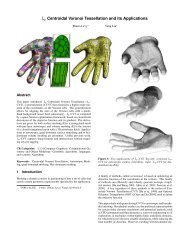
Texture Mapping Normal Mapping Detail Transfer<br />
Morphing <strong>Mesh</strong> Completion Editing<br />
Databases Remeshing Surface Fitting<br />
Figure 1.1: <strong>Parameterization</strong> Applications.<br />
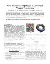
Figure 1.2: Application of parameterization: texture mapping (Least Squares Conformal<br />
Maps implemented in the Open-Source Blender modeler).<br />
2
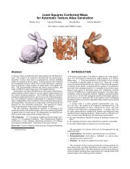
Figure 1.3: Application of parameterization: appearance-preserving simplication. All<br />
the details are encoded in a normal map, applied onto a dramatically simplied version<br />
of the model (1.5% of the original size).<br />
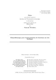
Figure 1.4: A global parameterization realizes an abstraction of the initial geometry.<br />
This abstraction can then be re-instanciated into alternative shape representations.<br />
3
than a 2D one. Such techniques are needed in order to model detail with complicated<br />
topology or detail that cannot be easily approximated locally by a height eld, such as<br />
sparsely interwoven structures or animal fur. The natural way to map details to surfaces<br />
is using planar parameterization.<br />
Detail Synthesis<br />
While the goal of texture mapping is to represent the complicated appearance of 3D<br />
objects, several methods make use of mesh parameterization to create the local detail<br />
necessary for a rich appearance. Such techniques can use as input at patches with<br />
sample detail, e.g. [Soler et al., 2002]; parametric or procedural models; or direct user<br />
input <strong>and</strong> editing [Carr <strong>and</strong> Hart, 2004]. The type of detail can be quite varied <strong>and</strong> the<br />
intermediate representations used to create it parallel the nal representations used to<br />
store it.<br />
Morphing <strong>and</strong> Detail Transfer<br />
A map between the surfaces of two objects allows the transfer of detail from one object<br />
to another (e.g. [Praun et al., 2001]), or the interpolation between the shape <strong>and</strong> appearance<br />
of several objects [Alexa, 2000; Kraevoy <strong>and</strong> Sheer, 2004; Schreiner et al., 2004].<br />
By varying the interpolation ratios over time, one can produce morphing animations.<br />
In spatially-varying <strong>and</strong> frequency-varying morphs, the rate of change can be dierent<br />
for dierent parts of the objects, or dierent frequency b<strong>and</strong>s (coarseness of the features<br />
being transformed) [Allen et al., 2003; Kraevoy <strong>and</strong> Sheer, 2004]. Such a map can<br />
either be computed directly or, as more commonly done, computed by mapping both<br />
object surfaces to a common domain. In addition to transferring the static appearance<br />
of surfaces, inter-surface parameterizations allow the transfer of animation data between<br />
shapes, either by transferring the local surface inuence from bones of an animation rig,<br />
or by directly transferring the local ane transformation of each triangle in the mesh<br />
[Sumner <strong>and</strong> Popovi¢, 2004].<br />
<strong>Mesh</strong> Completion<br />
<strong>Mesh</strong>es from range scans often contain holes <strong>and</strong> multiple components. Lévy [2003]<br />
uses planar parameterization to obtain the natural shape for hole boundaries <strong>and</strong> to<br />
triangulate those. In many cases, prior knowledge about the overall shape of the scanned<br />
models exists. For instance, for human scans, templates of a generic human shape are<br />
readily available. Allen et al. [2003] <strong>and</strong> Anguelov et al. [2005] use this prior knowledge to<br />
facilitate completion of scans by computing a mapping between the scan <strong>and</strong> a template<br />
human model. Kraevoy <strong>and</strong> Sheer [2005] develop a more generic <strong>and</strong> robust templatebased<br />
approach for completion of any type of scans. The techniques typically use an<br />
inter-surface parameterization between the template <strong>and</strong> the scan.<br />
4
<strong>Mesh</strong> Editing<br />
Editing operations often benet from a local parameterization between pairs of models.<br />
Biermann et al. [2002] use local parameterization to facilitate cut-<strong>and</strong>-paste transfer of<br />
details between models. They locally parameterize the regions of interest on the two<br />
models in 2D <strong>and</strong> overlap the two parameterizations. They use the parameterization to<br />
transfer shape properties from one model to the other. Lévy [2003] uses local parameterization<br />
for mesh composition in a similar manner. They compute an overlapping planar<br />
parameterization of the regions near the composition boundary on the input models <strong>and</strong><br />
use it to extract <strong>and</strong> smoothly blend shape information from the two models.<br />
Creation of Object Databases<br />
Once a large number of models are parameterized on a common domain one can perform<br />
an analysis determining the common factors between objects <strong>and</strong> their distinguishing<br />
traits. For example on a database of human shapes [Allen et al., 2003] the distinguishing<br />
traits may be gender, height, <strong>and</strong> weight. Objects can be compared against the database<br />
<strong>and</strong> scored against each of these dimensions, <strong>and</strong> the database can be used to create new<br />
plausible object instances by interpolation or extrapolation of existing ones.<br />
Remeshing<br />
There are many possible triangulations that represent the same shape with similar levels<br />
of accuracy. Some triangulation may be more desirable than others for dierent applications.<br />
For example, for numerical simulations on surfaces, triangles with a good aspect<br />
ratio (that are not too small or too skinny are important for convergence <strong>and</strong> numerical<br />
accuracy. One common way to remesh surfaces, or to replace one triangulation by another,<br />
is to parameterize the surface, then map a desirable, well-understood, <strong>and</strong> easy<br />
to create triangulation of the domain back to the original surface. For example, Gu<br />
et al. [2002] use a regular grid sampling of a planar square domain, while other methods,<br />
e.g. [Guskov et al., 2000] use regular subdivision (usually 1-to-4 triangle splits) on the<br />
faces of a simplicial domain. Such locally regular meshes can usually support the creation<br />
of smooth surfaces as the limit process of applying subdivision rules. To generate<br />
high quality triangulations, Desbrun et al. [2002] parameterize the input mesh in the<br />
plane <strong>and</strong> then use planar Delaunay triangulation to obtain a high quality remeshing of<br />
the surface. One problem these methods face is the appearance of visible discontinuities<br />
along the cuts created to facilitate the parameterization. Surazhsky <strong>and</strong> Gotsman [2003]<br />
avoid global parameterization, <strong>and</strong> instead use local parameterization to move vertices<br />
along the mesh as part of an explicit remeshing scheme. Recent methods such as [Ray<br />
et al., 2006] use global parameterization to generate a predominantly quadrilateral mesh<br />
directly on the 3D surface.<br />
5
<strong>Mesh</strong> Compression<br />
<strong>Mesh</strong> compression is used to compactly store or transmit geometric models. As with<br />
other data, compression rates are inversely proportional to the data entropy. Thus higher<br />
compression rates can be obtained when models are represented by meshes that are as<br />
regular as possible, both topologically <strong>and</strong> geometrically. Topological regularity refers<br />
to meshes where almost all vertices have the same degree. Geometric regularity implies<br />
that triangles are similar to each other in terms of shape <strong>and</strong> size <strong>and</strong> vertices are close<br />
to the centroid of their neighbors. Such meshes can be obtained by parameterizing the<br />
original objects <strong>and</strong> then remeshing with regular sampling patterns [Gu et al., 2002].<br />
The quality of the parameterization directly impacts the compression eciency.<br />
Surface Fitting<br />
One of the earlier applications of mesh parameterization is surface tting [Floater, 2000].<br />
Many applications in geometry processing require a smooth analytical surface to be<br />
constructed from an input mesh. A parameterization of the mesh over a base domain<br />
signicantly simplies this task. Earlier methods either parameterized the entire mesh<br />
in the plane or segmented it <strong>and</strong> parameterized each patch independently. More recent<br />
methods, e.g. [Li et al., 2006] focus on constructing smooth global parameterizations<br />
<strong>and</strong> use those for tting, achieving global continuity of the constructed surfaces.<br />
Modeling from Material Sheets<br />
While computer graphics focuses on virtual models, geometry processing has numerous<br />
real-world engineering applications. Particularly, planar mesh parameterization is an<br />
important tool when modeling 3D objects from sheets of material, ranging from garment<br />
modeling to metal forming or forging [Bennis et al., 1991; Julius et al., 2005]. All of<br />
these applications require the computation of planar patterns to form the desired 3D<br />
shapes. Typically, models are rst segmented into nearly developable charts, <strong>and</strong> these<br />
charts are then parameterized in the plane.<br />
Medical Visualization<br />
Complex geometric structures are often better visualized <strong>and</strong> analyzed by mapping the<br />
surface normal-map, color, <strong>and</strong> other properties to a simpler, canonical domain. One of<br />
the structures for which such mapping is particularly useful is the human brain [Hurdal<br />
et al., 1999; Haker et al., 2000]. Most methods for brain mapping use the fact that the<br />
brain has genus zero, <strong>and</strong> visualize it through spherical [Haker et al., 2000] or planar<br />
[Hurdal et al., 1999] parameterization.<br />
6
Chapter 2<br />
Dierential Geometry Primer<br />
Before we go into the details of how to compute a mesh parameterization <strong>and</strong> what to<br />
do with it, let us quickly review some of the basic properties from dierential geometry<br />
that will be essential for underst<strong>and</strong>ing the motivation behind the methods described<br />
later. For more details <strong>and</strong> proofs of these properties, we refer the interested reader<br />
to the st<strong>and</strong>ard literature on dierential geometry <strong>and</strong> in particular to the books by<br />
do Carmo [1976], Klingenberg [1978], Kreyszig [1991], <strong>and</strong> Morgan [1998].<br />
2.1 Basic Denitions<br />
Suppose that Ω ⊂ R 2 is some simply connected region (i.e., without any holes), for<br />
example,<br />
the unit square: Ω = {(u, v) ∈ R 2 : u, v ∈ [0, 1]}, or<br />
the unit disk: Ω = {(u, v) ∈ R 2 : u 2 + v 2 ≤ 1},<br />
<strong>and</strong> that the function f : Ω → R 3 is continuous <strong>and</strong> an injection (i.e., no two distinct<br />
points in Ω are mapped to the same point in R 3 ). We then call the image S of Ω under<br />
f a surface,<br />
S = f(Ω) = {f(u, v) : (u, v) ∈ Ω},<br />
<strong>and</strong> say that f is a parameterization of S over the parameter domain Ω. It follows from<br />
the denition of S that f is actually a bijection between Ω <strong>and</strong> S <strong>and</strong> thus admits to<br />
dene its inverse f −1 : S → Ω. Here are some examples:<br />
1. simple linear function:<br />
parameter domain: Ω = {(u, v) ∈ R 2 : u, v ∈ [0, 1]}<br />
surface: S = {(x, y, z) ∈ R 3 : x, y, z ∈ [0, 1], x + y = 1}<br />
parameterization: f(u, v) = (u, 1 − u, v)<br />
inverse: f −1 (x, y, z) = (x, z)<br />
7
2. cylinder:<br />
parameter domain: Ω = {(u, v) ∈ R 2 : u ∈ [0, 2π), v ∈ [0, 1]}<br />
surface: S = {(x, y, z) ∈ R 3 : x 2 + y 2 = 1, z ∈ [0, 1]}<br />
parameterization: f(u, v) = (cos u, sin u, v)<br />
inverse: f −1 (x, y, z) = (arccos x, z)<br />
3. paraboloid:<br />
parameter domain: Ω = {(u, v) ∈ R 2 : u, v ∈ [−1, 1]}<br />
surface: S = {(x, y, z) ∈ R 3 : x, y ∈ [−2, 2], z = 1 4 (x2 + y 2 )}<br />
parameterization: f(u, v) = (2u, 2v, u 2 + v 2 )<br />
inverse: f −1 (x, y, z) = ( x, y ) 2 2<br />
8
4. hemisphere (orthographic):<br />
parameter domain: Ω = {(u, v) ∈ R 2 : u 2 + v 2 ≤ 1}<br />
surface: S = {(x, y, z) ∈ R 3 : x 2 + y 2 + z 2 = 1, z ≥ 0}<br />
parameterization: f(u, v) = (u, v, √ 1 − u 2 − v 2 )<br />
inverse: f −1 (x, y, z) = (x, y)<br />
Having dened a surface S like that, we should note that the function f is by no<br />
means the only parameterization of S over Ω. In fact, given any bijection ϕ : Ω → Ω,<br />
it is easy to verify that the composition of f <strong>and</strong> ϕ, i.e., the function g = f ◦ ϕ, is<br />
a parameterization of S over Ω, too. For example, we can easily construct such a<br />
reparameterization ϕ from any bijection ρ : [0, 1] → [0, 1] by dening<br />
for the unit square: ϕ(u, v) = (ρ(u), ρ(v)), or<br />
for the unit disk: ϕ(u, v) = (uρ(u 2 + v 2 ), vρ(u 2 + v 2 )).<br />
In particular, taking the function ρ(x) = 2 <strong>and</strong> applying this reparameterization of<br />
1+x<br />
the unit disk to the parameterization of the hemisphere in the example above gives the<br />
following alternative parameterization:<br />
5. hemisphere (stereographic):<br />
parameter domain: Ω = {(u, v) ∈ R 2 : u 2 + v 2 ≤ 1}<br />
surface: S = {(x, y, z) ∈ R 3 : x 2 + y 2 + z 2 = 1, z ≥ 0}<br />
2u 2v<br />
parameterization: f(u, v) = ( , , 1−u2 −v 2<br />
1+u 2 +v 2 1+u 2 +v 2<br />
inverse: f −1 (x, y, z) = ( x , y<br />
)<br />
1+z 1+z<br />
1+u 2 +v 2 )<br />
9
2.2 Intrinsic Surface Properties<br />
Although the parameterization of a surface is not unique<strong>and</strong> we will later discuss how<br />
to get the best parameterization with respect to certain criteriait nevertheless is a<br />
very h<strong>and</strong>y thing to have as it allows to compute a variety of properties of the surface.<br />
For example, if f is dierentiable, then its partial derivatives<br />
f u = ∂f<br />
∂u<br />
<strong>and</strong><br />
f v = ∂f<br />
∂v<br />
span the local tangent plane <strong>and</strong> by simply taking their cross product <strong>and</strong> normalizing<br />
the result we get the surface normal<br />
n f =<br />
f u × f v<br />
‖f u × f v ‖ .<br />
To simplify the notation, we will often speak of f u <strong>and</strong> f v as the derivatives <strong>and</strong> of n f<br />
as the surface normal, but we should keep in mind that formally all three are functions<br />
from R 2 to R 3 . In other words, for any point (u, v) ∈ Ω in the parameter domain, the<br />
tangent plane at the surface point f(u, v) ∈ S is spanned by the two vectors f u (u, v)<br />
<strong>and</strong> f v (u, v), <strong>and</strong> n f (u, v) is the normal vector at this point 1 . Again, let us clarify this<br />
by considering two examples:<br />
1. For the simple linear function f(u, v) = (u, 1 − u, v) we get<br />
<strong>and</strong> further<br />
f u (u, v) = (1, −1, 0) <strong>and</strong> f v (u, v) = (0, 0, 1)<br />
n f (u, v) = ( −1 √<br />
2<br />
,<br />
1 √2 , 0),<br />
showing that the normal vector is constant for all points on S.<br />
2. For the parameterization of the cylinder, f(u, v) = (cos u, sin u, v), we get<br />
<strong>and</strong> further<br />
f u (u, v) = (− sin u, cos u, 0) <strong>and</strong> f v (u, v) = (0, 0, 1)<br />
n f (u, v) = (cos u, sin u, 0),<br />
showing that the normal vector at any point (x, y, z) ∈ S is just (x, y, 0).<br />
Note that in both examples the surface normal is independent of the parameterization.<br />
In fact, this holds for all surfaces <strong>and</strong> is therefore called an intrinsic property of the<br />
surface. Formally, we can also say that the surface normal is a function n : S → S 2 ,<br />
where S 2 = {(x, y, z) ∈ R 3 : x 2 + y 2 + z 2 = 1} is the unit sphere in R 3 , so that<br />
n(p) = n f (f −1 (p))<br />
1<br />
We tacitly assume that the parameterization is regular, i.e., f u <strong>and</strong> f v are always linearly independent<br />
<strong>and</strong> therefore n f is non-zero.<br />
10
for any p ∈ S <strong>and</strong> any parameterization f. As an exercise, you may want to verify this<br />
for the two alternative parameterizations of the hemisphere given above. Other intrinsic<br />
surface properties are the Gaussian curvature K(p) <strong>and</strong> the mean curvature H(p) as<br />
well as the total area of the surface A(S). To compute the latter, we need the rst<br />
fundamental form<br />
( ) ( )<br />
fu · f<br />
I f = u f u · f v E F<br />
= ,<br />
f v · f u f v · f v F G<br />
where the product between the partial derivatives is the usual dot product in R 3 . It<br />
follows immediately from the Cauchy-Schwarz inequality that the determinant of this<br />
symmetric 2 × 2 matrix is always non-negative, so that its square root is always real.<br />
The area of the surface is then dened as<br />
∫<br />
√<br />
A(S) = det If du dv.<br />
Ω<br />
Take, for example, the orthographic parameterization f(u, v) = (u, v, √ 1 − u 2 − v 2 )<br />
of the hemisphere over the unit disk. After some simplications we nd that<br />
det I f =<br />
1<br />
1 − u 2 − v 2<br />
<strong>and</strong> can compute the area of the hemisphere as follows:<br />
A(S) =<br />
=<br />
=<br />
∫ 1<br />
√<br />
1−v 2<br />
∫<br />
1<br />
−1 − √ 1−v 2<br />
∫ 1<br />
−1<br />
∫ 1<br />
−1<br />
= 2π,<br />
[<br />
arcsin<br />
π dv<br />
√ du dv<br />
1 − u2 − v2 ] √ 1−v<br />
u<br />
2<br />
√<br />
1 − v<br />
2<br />
− √ 1−v 2<br />
as expected. Of course we get the same result if we use the stereographic parameterization,<br />
<strong>and</strong> you may want to try that as an exercise.<br />
In order to compute the curvatures we must rst assume the parameterization to be<br />
twice dierentiable, so that its second order partial derivatives<br />
f uu = ∂2 f<br />
∂u 2 ,<br />
dv<br />
f uv = ∂2 f<br />
∂u∂v , <strong>and</strong> f vv = ∂2 f<br />
∂v 2<br />
are well dened. Taking the dot products of these derivatives with the surface normal<br />
then gives the symmetric 2 × 2 matrix that is known as the second fundamental form<br />
( ) ( )<br />
fuu · n<br />
II f =<br />
f f uv · n f L M<br />
= .<br />
f uv · n f f vv · n f M N<br />
11
Gaussian <strong>and</strong> mean curvature are nally dened as the determinant <strong>and</strong> half the trace<br />
of the matrix I −1<br />
f<br />
II f, respectively:<br />
<strong>and</strong><br />
K = det(I −1<br />
f<br />
II f) = det II f<br />
= LN − M 2<br />
det I f EG − F 2<br />
H = 1 2 trace(I−1 f<br />
II f) =<br />
LG − 2MF + NE<br />
.<br />
2(EG − F 2 )<br />
For example, carrying out these computations reveals that the curvatures are constant<br />
for most of the surfaces from above:<br />
simple linear function: K = 0, H = 0,<br />
cylinder: K = 0, H = 1 2 ,<br />
hemisphere: K = 1, H = −1.<br />
As an exercise, show that the curvatures at any point p = (x, y, z) of the paraboloid<br />
from above are K(p) = 1 <strong>and</strong> H(p) = 2+z .<br />
4(1+z) 2 4(1+z) 3/2<br />
2.3 Metric Distortion<br />
Apart from these intrinsic surface properties, there are others that depend on the parameterization,<br />
most importantly the metric distortion. Consider, for example, the two<br />
parameterizations of the hemisphere above. In both cases, the image of the surface on<br />
the right is overlaid by a regular grid, which actually is the image of the corresponding<br />
grid in the parameter domain shown on the left. You will notice that the surface grid<br />
looks more regular for the stereographic than for the orthographic projection <strong>and</strong> that<br />
the latter considerably stretches the grid in the radial direction near the boundary.<br />
To better underst<strong>and</strong> this kind of stretching, let us see what happens to the surface<br />
point f(u, v) as we move a tiny little bit away from (u, v) in the parameter domain. If<br />
we denote this innitesimal parameter displacement by (∆u, ∆v), then the new surface<br />
point f(u + ∆u, v + ∆v) is approximately given by the rst order Taylor expansion ˜f of<br />
f around (u, v),<br />
˜f(u + ∆u, v + ∆v) = f(u, v) + f u (u, v)∆u + f v (u, v)∆v.<br />
This linear function maps all points in the vicinity of u = (u, v) into the tangent plane<br />
T p at p = f(u, v) ∈ S <strong>and</strong> transforms circles around u into ellipses around p (see<br />
Figure 2.1). The latter property becomes obvious if we write the Taylor expansion more<br />
compactly as<br />
˜f(u + ∆u, v + ∆v) = p + J f (u) ( ∆u<br />
∆v)<br />
,<br />
where J f = (f u f v ) is the Jacobian of f, i.e. the 3 × 2 matrix with the partial derivatives<br />
of f as column vectors. Then using the singular value decomposition of the Jacobian,<br />
(<br />
σ1<br />
)<br />
J f = UΣV T 0<br />
= U V T ,<br />
12<br />
0 σ 2<br />
0 0
Figure 2.1: First order Taylor expansion ˜f of the parameterization f.<br />
Figure 2.2: SVD decomposition of the mapping ˜f.<br />
with singular values σ 1 ≥ σ 2 > 0 <strong>and</strong> orthonormal matrices U ∈ R 3×3 <strong>and</strong> V ∈ R 2×2<br />
with column vectors U 1 , U 2 , U 3 , <strong>and</strong> V 1 , V 2 , respectively, we can split up the linear transformation<br />
˜f as shown in Figure 2.2:<br />
1. The transformation V T rst rotates all points around u such that the vectors V 1<br />
<strong>and</strong> V 2 are in alignment with the u- <strong>and</strong> the v-axes afterwards.<br />
2. The transformation Σ then stretches everything by the factor σ 1 in the u- <strong>and</strong> by<br />
σ 2 in the v-direction.<br />
3. The transformation U nally maps the unit vectors (1, 0) <strong>and</strong> (0, 1) to the vectors<br />
U 1 <strong>and</strong> U 2 in the tangent plane T p at p.<br />
As a consequence, any circle of radius r around u will be mapped to an ellipse with<br />
semi-axes of length rσ 1 <strong>and</strong> rσ 2 around p <strong>and</strong> the orthonormal frame [V 1 , V 2 ] is mapped<br />
to the orthogonal frame [σ 1 U 1 , σ 2 U 2 ].<br />
This transformation of circles into ellipses is called local metric distortion of the<br />
parameterization as it shows how f behaves locally around some parameter point u ∈ Ω<br />
<strong>and</strong> the corresponding surface point p = f(u) ∈ S. Moreover, all information about<br />
this local metric distortion is hidden in the singular values σ 1 <strong>and</strong> σ 2 . For example, if<br />
both values are identical, then J f is just a rotation plus uniform scaling <strong>and</strong> f does not<br />
distort angles around u. Likewise, if the product of the singular values is 1, then the<br />
area of any circle in the parameter domain is identical to the area of the corresponding<br />
ellipse in the tangent plane <strong>and</strong> we say that f is locally area-preserving.<br />
Computing the singular values directly is a bit tedious, so that we better resort to<br />
the fact that the singular values of any matrix A are the square roots of the eigenvalues<br />
of the matrix A T A. In our case, the matrix J f T J f is an old acquaintance, namely the<br />
13
st fundamental form,<br />
J f T J f =<br />
(<br />
fu<br />
T<br />
f v<br />
T<br />
)<br />
(f u f v ) = I f =<br />
( ) E F<br />
,<br />
F G<br />
<strong>and</strong> we can easily compute the two eigenvalues λ 1 <strong>and</strong> λ 2 of this symmetric matrix by<br />
using the nifty little formula<br />
λ 1,2 = 1 2(<br />
(E + G) ±<br />
√<br />
4F<br />
2<br />
+ (E − G) 2) .<br />
We now summarize the main properties that a parameterization can have locally:<br />
f is isometric or length-preserving ⇐⇒ σ 1 = σ 2 = 1 ⇐⇒ λ 1 = λ 2 = 1,<br />
f is conformal or angle-preserving ⇐⇒ σ 1 = σ 2 ⇐⇒ λ 1 = λ 2 ,<br />
f is equiareal or area-preserving ⇐⇒ σ 1 σ 2 = 1 ⇐⇒ λ 1 λ 2 = 1.<br />
Obviously, any isometric mapping is conformal <strong>and</strong> equiareal, <strong>and</strong> every mapping that<br />
is conformal <strong>and</strong> equiareal is also isometric, in short,<br />
isometric ⇐⇒ conformal + equiareal.<br />
Thus equipped, let us go back to the examples above <strong>and</strong> check their properties:<br />
1. simple linear function:<br />
parameterization: f(u, v) = (u, 1 − u, v)<br />
)<br />
Jacobian: J f =<br />
( 1 0<br />
−1 0<br />
0 1<br />
rst fundamental form: I f = ( 2 0<br />
0 1<br />
eigenvalues: λ 1 = 2, λ 2 = 1<br />
This parameterization is neither conformal nor equiareal.<br />
2. cylinder:<br />
parameterization: f(u, v) = (cos u, sin u, v)<br />
)<br />
Jacobian: J f =<br />
rst fundamental form: I f = ( 1 0<br />
0 1<br />
This parameterization is isometric.<br />
)<br />
( cos u 0<br />
− sin u 0<br />
0 1<br />
eigenvalues: λ 1 = 1, λ 2 = 1<br />
14<br />
)
3. paraboloid:<br />
parameterization: f(u, v) = (2u, 2v, u 2 + v 2 )<br />
)<br />
Jacobian: J f =<br />
( 2 0<br />
0 2<br />
2u 2v<br />
rst fundamental form: I f = ( )<br />
4+4u 2 4uv<br />
4uv 4+4v 2<br />
eigenvalues: λ 1 = 4, λ 2 = 4(1 + u 2 + v 2 )<br />
This mapping is not equiareal <strong>and</strong> conformal only at (u, v) = (0, 0).<br />
4. hemisphere (orthographic):<br />
parameterization: f(u, v) = (u, v, 1) with d = √ 1<br />
d 1−u 2 −v 2<br />
( 1 0<br />
)<br />
Jacobian: J f = 0 1<br />
−ud −vd<br />
rst fundamental form: I f = ( 1+u 2 d 2 uvd 2<br />
uvd 2 1+v 2 d 2 )<br />
eigenvalues: λ 1 = 1, λ 2 = d 2<br />
This mapping is isometric at (u, v) = (0, 0), but neither conformal nor equiareal<br />
elsewhere.<br />
5. hemisphere (stereographic):<br />
parameterization: f(u, v) = (2ud, 2vd, (1 − u 2 − v 2 )d) with d =<br />
1<br />
Jacobian: J f =<br />
( 2d−4u 2 d 2 −4uvd 2<br />
rst fundamental form: I f = ( 4d 2 0<br />
0 4d 2 )<br />
)<br />
−4uvd 2 2d−4v 2 d 2<br />
eigenvalues: λ 1 = 4d 2 , λ 2 = 4d 2<br />
1+u 2 +v 2<br />
This mapping is always conformal, but equiareal <strong>and</strong> thus isometric only at the<br />
boundary of Ω, i.e., for u 2 + v 2 = 1.<br />
It turns out that the only parameterization that is optimal in the sense that it is<br />
isometric everywhere <strong>and</strong> thus does not introduce any distortion at all is the one for the<br />
cylinder. In fact, it was shown by Gauÿ [1827] that a globally isometric parameterization<br />
exists only for developable surfaces like planes, cones, <strong>and</strong> cylinders with vanishing<br />
Gaussian curvature K(p) = 0 at all surface points p ∈ S. As an exercise, you can try<br />
to nd such a globally isometric parameterization for the planar surface patch from the<br />
rst example.<br />
Other interesting parameterizations are those that are globally conformal like the<br />
stereographic projection for the hemisphere, <strong>and</strong> it was shown by Riemann [1851] that<br />
15
such a parameterization exists for any surface that is topologically equivalent to a disk<br />
<strong>and</strong> any simply connected parameter domain.<br />
More generally, the best parameterization f of a surface S over a parameter domain<br />
Ω is found as follows. We rst need a bivariate non-negative function E : R 2 + → R +<br />
that measures the local distortion of a parameterization with singular values σ 1 <strong>and</strong><br />
σ 2 . Usually, this function has a global minimum at (1, 1) so as to favour isometry, but<br />
depending on the application, it may also be dened such that the minimal value is<br />
taken along the whole line (x, x) for x ∈ R + , for example, if conformal mappings shall<br />
be preferred. The overall distortion of a particular parameterization f is then measured<br />
by simply averaging the local distortion over the whole domain,<br />
∫<br />
E(f) =<br />
Ω<br />
/<br />
E(σ 1 (u, v), σ 2 (u, v)) du dv A(Ω),<br />
<strong>and</strong> the best parameterization with respect to E is then found by minimizing E(f) over<br />
the space of all admissible parameterizations.<br />
16
Chapter 3<br />
Barycentric Mappings<br />
In many applications, <strong>and</strong> in particular in computer graphics, it is nowadays common<br />
to work with piecewise linear surfaces in the form of triangle meshes, <strong>and</strong> we will mainly<br />
stick to this type of surface for the remainder of these course notes.<br />
3.1 Triangle <strong>Mesh</strong>es<br />
As in the previous chapter, let us denote points in R 3 by p = (x, y, z) <strong>and</strong> points in<br />
R 2 by u = (u, v). An edge is then dened as the convex hull of (or, equivalently, the<br />
line segment between) two distinct points <strong>and</strong> a triangle as the convex hull of three<br />
non-collinear points. We will denote edges <strong>and</strong> triangles in R 3 with capital letters <strong>and</strong><br />
those in R 2 with small letters, for example, e = [u 1 , u 2 ] <strong>and</strong> T = [p 1 , p 2 , p 3 ].<br />
A triangle mesh S T is the union of a set of surface triangles T = {T 1 , . . . , T m } which<br />
intersect only at common edges E = {E 1 , . . . , E l } <strong>and</strong> vertices V = {p 1 , . . . , p n+b }. More<br />
specically, the set of vertices consists of n interior vertices V I = {p 1 , . . . , p n } <strong>and</strong> b<br />
boundary vertices V B = {p n+1 , . . . , p n+b }. Two distinct vertices p i , p j ∈ V are called<br />
neighbours, if they are the end points of some edge E = [p i , p j ] ∈ E, <strong>and</strong> for any p i ∈ V<br />
we let N i = {j : [p i , p j ] ∈ E} be the set of indices of all neighbours of p i .<br />
A parameterization f of S T is usually specied the other way around, that is, by<br />
dening the inverse parameterization g = f −1 . This mapping g is uniquely determined<br />
by specifying the parameter points u i = g(p i ) for each vertex p i ∈ V <strong>and</strong> dem<strong>and</strong>ing that<br />
g is continuous <strong>and</strong> linear for each triangle. In this setting, g| T is the linear map from a<br />
surface triangle T = [p i , p j , p k ] to the corresponding parameter triangle t = [u i , u j , u k ]<br />
<strong>and</strong> f| t = (g| T ) −1 is the inverse linear map from t to T . The parameter domain Ω nally<br />
is the union of all parameter triangles (see Figure 3.1).<br />
3.2 <strong>Parameterization</strong> by Ane Combinations<br />
A rather simple idea for constructing a parameterization of a triangle mesh is based on<br />
the following physical model. Imagine that the edges of the triangle mesh are springs<br />
that are connected at the vertices. If we now x the boundary of this spring network<br />
somewhere in the plane, then the interior of this network will relax in the energetically<br />
17
S T<br />
g| T<br />
Ω<br />
t<br />
T<br />
f| t<br />
Figure 3.1: <strong>Parameterization</strong> of a triangle mesh.<br />
most ecient conguration, <strong>and</strong> we can simply assign the positions where the joints of<br />
the network have come to rest as parameter points.<br />
If we assume each spring to be ideal in the sense that the rest length is zero <strong>and</strong> the<br />
potential energy is just 1 2 Ds2 , where D is the spring constant <strong>and</strong> s the length of the<br />
spring, then we can formalize this approach as follows. We rst specify the parameter<br />
points u i = (u i , v i ), i = n + 1, . . . , n + b for the boundary vertices p i ∈ V B of the mesh<br />
in some way (see Section 3.4). Then we minimize the overall spring energy<br />
E = 1 2<br />
n∑ ∑<br />
i=1<br />
j∈N i<br />
1<br />
2 D ij‖u i − u j ‖ 2 ,<br />
where D ij = D ji is the spring constant of the spring between p i <strong>and</strong> p j , with respect<br />
to the unknown parameter positions u i = (u i , v i ) for the interior points 1 . As the partial<br />
derivative of E with respect to u i is<br />
the minimum of E is obtained if<br />
∑<br />
∂E<br />
∂u i<br />
= ∑ j∈N i<br />
D ij (u i − u j ),<br />
j∈N i<br />
D ij u i = ∑ j∈N i<br />
D ij u j<br />
holds for all i = 1, . . . , n. This is equivalent to saying that each interior parameter point<br />
u i is an ane combination of its neighbours,<br />
u i = ∑ j∈N i<br />
λ ij u j , (3.1)<br />
with normalized coecients<br />
that obviously sum to 1.<br />
λ ij = D ij<br />
/ ∑<br />
k∈N i<br />
D ik<br />
1<br />
The additional factor 1 2<br />
appears because summing up the edges in this way counts every edge twice.<br />
18
By separating the parameter points for the interior <strong>and</strong> the boundary vertices in the<br />
sum on the right h<strong>and</strong> side of (3.1) we get<br />
u i −<br />
∑<br />
λ ij u j =<br />
∑<br />
λ ij u j ,<br />
j∈N i ,j≤n<br />
j∈N i ,j>n<br />
<strong>and</strong> see that computing the coordinates u i <strong>and</strong> v i of the interior parameter points u i<br />
requires to solve the linear systems<br />
AU = Ū <strong>and</strong> AV = ¯V , (3.2)<br />
where U = (u 1 , . . . , u n ) <strong>and</strong> V = (v 1 , . . . , v n ) are the column vectors of unknown coordinates,<br />
Ū = (ū 1, . . . , ū n ) <strong>and</strong> ¯V = (¯v 1 , . . . , ¯v n ) are the column vectors with coecients<br />
ū i =<br />
∑<br />
λ ij u j <strong>and</strong> ¯v i = ∑<br />
λ ij v j<br />
j∈N i ,j>n<br />
<strong>and</strong> A = (a ij ) i,j=1,...,n<br />
is the n × n matrix with elements<br />
⎧<br />
⎪⎨ 1 if i = j,<br />
a ij = −λ ij if j ∈ N i ,<br />
⎪⎩<br />
0 otherwise.<br />
j∈N i ,j>n<br />
Methods for eciently solving these systems are described in Chapter 10 of these course<br />
notes.<br />
3.3 Barycentric Coordinates<br />
The question remains how to choose the spring constants D ij in the spring model, or<br />
more generally, the normalized coecients λ ij in (3.1). The simplest choice of constant<br />
spring constants D ij = 1 goes back to the work of Tutte [1960, 1963] who used it in<br />
a more abstract graph-theoretic setting to compute straight line embeddings of planar<br />
graphs, <strong>and</strong> the idea of taking spring constants that are proportional to the lengths of<br />
the corresponding edges in the triangle mesh was used by Greiner <strong>and</strong> Hormann [1997].<br />
A main drawback of both approaches is that they do not fulll the following minimum<br />
requirement that we should expect from any parameterization method.<br />
Linear reproduction: Suppose that S T is contained in a plane so that its vertices<br />
have coordinates p i = (x i , y i , 0) with respect to some appropriately chosen orthonormal<br />
coordinate frame. Then a globally isometric (<strong>and</strong> thus optimal) parameterization can be<br />
dened by just using the local coordinates x i = (x i , y i ) as parameter points themselves,<br />
that is, by setting u i = x i for i = 1, . . . , n + b. As the overall parameterization then is<br />
a linear function, we say that a parameterization method has linear reproduction if it<br />
produces such an isometric mapping in this setting.<br />
19
Figure 3.2: Notation for the construction of barycentric coordinates.<br />
In the setting from the previous section, linear reproduction can be achieved if the<br />
parameter points for the boundary vertices are set correctly <strong>and</strong> the values λ ij are chosen<br />
such that<br />
x i = ∑ ∑<br />
λ ij x j <strong>and</strong><br />
j∈N i<br />
j∈N i<br />
λ ij = 1<br />
for all interior vertices. Values λ ij with both these properties are also called barycentric<br />
coordinates of x i with respect to its neighbours x j , j ∈ N i . If some x i has exactly three<br />
neighbours, then the λ ij are uniquely dened <strong>and</strong> these barycentric coordinates inside<br />
triangles actually have many useful applications in computer graphics (e.g., Gouraud <strong>and</strong><br />
Phong shading, ray-triangle-intersection), geometric modelling (e.g., triangular Bézier<br />
patches, splines over triangulations), <strong>and</strong> many other elds (e.g., the nite element<br />
method, terrain modelling).<br />
For polygons with more than three vertices, the barycentric coordinates of a point<br />
in the interior are, however, not unique anymore <strong>and</strong> there are several ways of dening<br />
them. The most popular of them can all be described in a common framework [Floater<br />
et al., 2006] that we shall briey review. For any interior point x i <strong>and</strong> one of its neighbours<br />
x j let r ij = ‖x i − x j ‖ be the length of the edge e ij = [x i , x j ] between the two<br />
points <strong>and</strong> let the angles at the corners of the triangles adjacent to e ij be denoted as<br />
shown in Figure 3.2. The barycentric coordinates λ ij of x i with respect its neighbours<br />
x j , j ∈ N i can then be computed by the normalization λ ij = w ij<br />
/ ∑k∈N i<br />
w ik from any<br />
of the following homogeneous coordinates w ij .<br />
• Wachspress coordinates: The earliest generalization of barycentric coordinates goes<br />
back to Wachspress [1975] who suggested to set<br />
w ij = cot α ji + cot β ij<br />
r ij<br />
2<br />
.<br />
While he was mainly interested in applying these coordinates in nite element<br />
methods, Desbrun et al. [2002] used them for parameterizing triangle meshes <strong>and</strong><br />
Meyer et al. [2002] for interpolating e.g. colour values inside convex polygons.<br />
Moreover, a simple geometric construction of these coordinates was given by Ju<br />
et al. [2005b].<br />
20
p 1 = (3,0,1)<br />
p 5 = (-1,1,0)<br />
p 4 = (1,1,0)<br />
p 2 = (-1,-1,0) p 3 = (1,-1,0)<br />
Figure 3.3: Example of a triangle mesh for which only the barycentric mapping with<br />
mean value coordinates is a bijection.<br />
• Discrete harmonic coordinates : Another type of barycentric coordinates that stem<br />
from nite element methods <strong>and</strong> actually arise from the st<strong>and</strong>ard piecewise linear<br />
approximation to the Laplace equation are given by<br />
w ij = cot γ ij + cot γ ji .<br />
In the context of mesh parameterization, these coordinates were rst used by Eck<br />
et al. [1995], but they have also been used to compute discrete minimal surfaces<br />
[Pinkall <strong>and</strong> Polthier, 1993].<br />
• Mean value coordinates: By discretizing the mean value theorem, Floater [2003a]<br />
found yet another set of barycentric coordinates with<br />
w ij = tan α ij<br />
+ tan β ji<br />
2 2<br />
.<br />
r ij<br />
While his main application was mesh parameterization, Hormann <strong>and</strong> Tarini [2004]<br />
<strong>and</strong> Hormann <strong>and</strong> Floater [2006] later showed that they have many other useful<br />
applications, in particular in computer graphics.<br />
The beauty of all three choices is that the weights w ij depend on angles <strong>and</strong> distances<br />
only, so that they can not only be computed if x i <strong>and</strong> its neighbours are coplanar, but<br />
more generally for any interior vertex p i ∈ V I of a triangle mesh if these angles <strong>and</strong><br />
distances are just taken from the triangles around p i . Of course, an alternative approach<br />
that was introduced by Floater [1997] is to locally atten the one-ring of triangles around<br />
p i into the plane, e.g. with an exponential map, <strong>and</strong> then to compute the weights w ij<br />
from this planar conguration.<br />
A triangle mesh parameterization that is computed by solving the linear systems (3.2)<br />
with any set of barycentric coordinates λ ij is called a barycentric mapping <strong>and</strong> obviously<br />
has the linear reproduction property, provided that an appropriate method for computing<br />
the parameter points for the boundary vertices, e.g. mapping them to the least squares<br />
plane (see Section 3.4), is used.<br />
Despite this property, it may happen that a barycentric mapping, when constructed<br />
for a non-planar mesh, gives an unexpected result, as the simple example in Figure 3.3<br />
21
x 6 = (-1,1)<br />
x 3 = (1/3,0)<br />
x 7 = (-1/3,0)<br />
x 5 = (1,0)<br />
x 2 = (0,0)<br />
x 4 = (-1,-1)<br />
x 1 = (-1/5,0)<br />
Figure 3.4: Example of a triangle mesh for which the linear system with Wachspress<br />
coordinates is singular.<br />
illustrates. If we use u 2 = (−1, −1), u 3 = (1, −1), u 4 = (1, 1), u 5 = (−1, 1) as parameter<br />
points for the four boundary vertices <strong>and</strong> compute the barycentric weights λ 12 , λ 13 , λ 14 ,<br />
λ 15 with the formulas described above, then we get the following positions for u 1 :<br />
Wachspress coordinates: u 1 = (−35.1369, 0),<br />
discrete harmonic coordinates: u 1 = (2.1138, 0),<br />
mean value coordinates: u 1 = (0.4538, 0).<br />
That is, only the mean value coordinates yield a position for u 1 that is contained in<br />
the convex hull of the other four parameter points, <strong>and</strong> using the other coordinates will<br />
create parameter triangles that overlap, thus violating the bijectivity property that any<br />
parameterization should have.<br />
The reason behind this behaviour is that the Wachspress <strong>and</strong> discrete harmonic coordinates<br />
can assume negative values in certain congurations like the one in Figure 3.3,<br />
whereas the mean values coordinates are always positive. And while overlapping triangles<br />
may occur for negative weights, this never happens if all weights are positive <strong>and</strong><br />
the parameter points of the boundary vertices form a convex shape. The latter fact has<br />
rst been proven by Tutte [1963] for the special case of λ ij = 1/η i where η i = #N i is<br />
the number of p i 's neighbours, which are not true barycentric coordinates, but Floater<br />
[1997] observed that the proof carries over to arbitrary positive weights λ ij . Recently,<br />
Gortler et al. [2006] could even show that the restriction to a convex boundary can be<br />
considerably relaxed, but this requires to solve a non-linear problem.<br />
Another important aspect concerns the solvability of the linear systems (3.2) <strong>and</strong> it<br />
has been shown that the matrix A is always guaranteed to be non-singular for discrete<br />
harmonic [Pinkall <strong>and</strong> Polthier, 1993] <strong>and</strong> mean value coordinates [Floater, 1997]. For<br />
Wachspress coordinates, however, it may happen that the sum of homogeneous coordinates<br />
W i = ∑ k∈N i<br />
w ik is zero so that the normalized coordinates λ ij <strong>and</strong> thus the matrix<br />
A are not even well-dened. In the example shown in Figure 3.4 this actually happens<br />
for all interior vertices x 1 , x 2 , x 3 . But even if we skip the normalization <strong>and</strong> try to solve<br />
the equivalent <strong>and</strong> well-dened homogeneous systems W AU = W Ū <strong>and</strong> W AV = W ¯V<br />
with W = diag(W 1 , . . . , W n ) instead, we nd)<br />
that the matrix W A is singular in this<br />
particular example, namely W A =<br />
.<br />
( 0 −50 0<br />
40 0 −24<br />
0 18 0<br />
22
3.4 The Boundary Mapping<br />
The rst step in constructing a barycentric mapping is to choose the parameter points<br />
for the boundary vertices <strong>and</strong> the simplest way of doing it is to just project the boundary<br />
vertices into the plane that ts the boundary vertices best in a least squares sense.<br />
However, for meshes with a complex boundary, this simple procedure may lead to undesirable<br />
fold-overs in the boundary polygon <strong>and</strong> cannot be used. In general, there are<br />
two issues to take into account here: (1) choosing the shape of the boundary of the<br />
parameter domain <strong>and</strong> (2) choosing the distribution of the parameter points around the<br />
boundary.<br />
Choosing the shape<br />
In many applications, it is sucient (or even desirable) to take a rectangle or a circle<br />
as parameter domain, with the advantage that such a convex shape guarantees the<br />
bijectivity of the parameterization if positive barycentric coordinates like the mean value<br />
coordinates are used to compute the parameter points for the interior vertices. The<br />
convexity restriction may, however, generate big distortions near the boundary when<br />
the boundary of the triangle mesh S T does not resemble a convex shape. One practical<br />
solution to avoid such distortions is to build a virtual boundary, i.e., to augment the<br />
given mesh with extra triangles around the boundary so as to construct an extended<br />
mesh with a nice boundary. This approach has been successfully used by Lee et al.<br />
[2002], <strong>and</strong> Kós <strong>and</strong> Várady [2003].<br />
Choosing the distribution<br />
The usual procedure mentioned in the literature is to use a simple univariate parameterization<br />
method such as chord length [Ahlberg et al., 1967] or centripetal parameterization<br />
[Lee, 1989] for placing the parameter points either around the whole boundary, or along<br />
each side of the boundary when working with a rectangular domain [Hormann, 2001,<br />
Section 1.2.5].<br />
Despite these heuristics working pretty well in some cases, having to x the boundary<br />
vertices may be a severe limitation in others <strong>and</strong> the next chapter studies parameterization<br />
methods that can include the position of the boundary parameter points in the<br />
optimization process <strong>and</strong> thus yield parameterizations with less distortion.<br />
23
Chapter 4<br />
Setting the Boundary Free<br />
As explained in the previous section, Tutte's theorem combined with mean value weights<br />
provides a provably correct way of constructing a valid parameterization for a disk-like<br />
surface. However, for some surfaces, the necessity to x the boundary on a convex<br />
polygon may be problematic (c.f. Figure 4.1), for the following reasons : (1) in general,<br />
it is dicult to nd a natural way of xing the border on a convex polygon, <strong>and</strong><br />
(2) for some surfaces, the shape of the boundary is far from convex. Therefore the<br />
obtained parameterization shows high deformations. Even if one can imagine dierent<br />
ways of improving the result shown in the Figure, the so-obtained parameterization will<br />
be probably not as good as the one shown in Figure 4.1-C, that better matches what<br />
a tanner would expect for such a mesh. For these reasons, the next section studies<br />
the methods that can construct parameterizations with free boundaries, that minimize<br />
deformations in a similar way. We start by giving an intuition of how to use the notions<br />
from dierential geometry explained in Chapter 2 in our context of parameterization<br />
with free boundaries.<br />
4.1 Deformation analysis<br />
To see how to apply the theoretic concepts explained in Chapter 2, we rst need to grasp<br />
their intuitive meaning.<br />
4.1.1 The Jacobian matrix<br />
The rst derivatives of the parameterization are involved in deformation analysis, it is<br />
then necessary to have an intuition of their geometric meaning. In physics, material point<br />
mechanics studies the movement of an object, approximated by a point p, when forces<br />
are applied to it. The trajectory is the curve described by the point p when t varies from<br />
t 0 to t 1 , where t denotes time. The function putting a given time t in correspondence<br />
with the position p(t) = {x(t), y(t), z(t)} of the point p is a parameterization of the<br />
trajectory, i.e., a parameterization of a curve. It is well known that the vector of the<br />
derivatives v(t) = ∂p/∂t = {∂x/∂t, ∂y/∂t, ∂z/∂t} corresponds to the speed of p at<br />
time t.<br />
24
Figure 4.1: A: a mesh cut in a way that makes it homeomorphic to a disk, using the<br />
seamster algorithm [Sheer <strong>and</strong> Hart, 2002]; B: Tutte-Floater parameterization obtained<br />
by xing the border on a square; C: parameterization obtained with a free-boundary<br />
parameterization [Sheer <strong>and</strong> de Sturler, 2001].<br />
v<br />
RI 2<br />
u 0<br />
w<br />
dv du<br />
Ω<br />
v 0<br />
x(u,v)<br />
u<br />
IR<br />
3<br />
Cu<br />
Cv<br />
C w<br />
∂x<br />
∂v<br />
∂x<br />
∂u<br />
w’<br />
S<br />
Figure 4.2: Elementary displacements from a point (u, v) of Ω along the u <strong>and</strong> the v axes<br />
are transformed into the tangent vectors to the iso-u <strong>and</strong> iso-v curves passing through<br />
the point f(u, v)<br />
25
As shown in Figure 4.2, we consider now a function f : (u, v) ↦→ (x, y, z), putting a<br />
subspace Ω of R 2 in one-to-one correspondence with a surface S of R 3 . The scalars (u, v)<br />
are the coordinates in parameter space. In the case of a curve parameterization, the<br />
curve is described by a single parameter t. In contrast, in our case, we consider a surface<br />
parameterization f(u, v) = {x(u, v), y(u, v), z(u, v)}, <strong>and</strong> there are two parameters, u<br />
<strong>and</strong> v. Therefore, at a given point (u 0 , v 0 ) of the parameter space Ω, there are two<br />
speed vectors to consider: f u = (∂f/∂u)(u 0 , v 0 ) <strong>and</strong> f v = (∂f/∂v)(u 0 , v 0 ). It is easy to<br />
check that f u is the speed vector of the curve C u : t ↦→ f(u 0 + t, v 0 ) at X (u 0 , v 0 ) <strong>and</strong><br />
that f v is the speed vector of the curve C v : t ↦→ f(u 0 , v 0 + t). The curve C u (resp.<br />
C v ) is the iso-u (resp. the iso-v) curve passing through f(u 0 , v 0 ), i.e. the image through<br />
f of the line of equation u = u 0 (resp. v = v 0 ).<br />
4.1.2 The 1 st fundamental form <strong>and</strong> the anisotropy ellipse<br />
At that point, one may think that the information provided by the two vectors f u (u 0 , v 0 )<br />
<strong>and</strong> f v (u 0 , v 0 ) is not sucient to characterize the distortions between Ω <strong>and</strong> S in the<br />
neighborhood of (u 0 , v 0 ) <strong>and</strong> f(u 0 , v 0 ). In fact, they can be used to compute how an<br />
arbitrary vector w = (a, b) in parameter space is transformed into a vector w ′ in the<br />
neighborhood of (u 0 , v 0 ). In other words, we want to compute the speed vector w ′ =<br />
∂f(u 0 + t.a, v 0 + t.b)/∂t of the curve corresponding to the image of the straight line<br />
(u, v) = (u 0 , v 0 ) + t.w. The vector w ′ , i.e. the tangent to the curve C w , can be simply<br />
computed by applying the chain rule, <strong>and</strong> one can check that it can be computed from<br />
the derivatives of f as follows : w ′ = af u (u 0 , v 0 ) + bf v (u 0 , v 0 ). The vector w ′ is referred<br />
to as the directional derivative of f at (u 0 , v 0 ) relative to the direction w.<br />
In matrix form, w ′ is obtained by w ′ = J(u 0 , v 0 )w, where J(u 0 , v 0 ) is the matrix of<br />
all the partial derivatives of f:<br />
⎡<br />
J(u 0 , v 0 ) =<br />
⎢<br />
⎣<br />
∂x<br />
(u ∂u 0, v 0 )<br />
∂y<br />
∂u (u 0, v 0 )<br />
∂z<br />
(u ∂u 0, v 0 )<br />
∂x<br />
(u ∂v 0, v 0 )<br />
∂y<br />
∂v (u 0, v 0 )<br />
∂z<br />
(u ∂v 0, v 0 )<br />
⎤<br />
[<br />
]<br />
⎥<br />
⎦ = f u (u 0 , v 0 ) . f v (u 0 , v 0 )<br />
(4.1)<br />
As already said in Chapter 2, the matrix J(u 0 , v 0 ) is referred to as the Jacobian<br />
matrix of f at (u 0 , v 0 ).<br />
The notion of directional derivative makes it possible to know what an elementary<br />
displacement w from a point (u 0 , v 0 ) in parameter space becomes when it is transformed<br />
by the function f. The Jacobian matrix helps also computing dot products <strong>and</strong> vector<br />
norms onto the surface S. This can be done using the matrix J T J, referred to as the 1 st<br />
fundamental form of f, also described in the dierential geometry section. This matrix<br />
is denoted by I, <strong>and</strong> dened by :<br />
⎡<br />
⎤<br />
f u · f u f u · f v<br />
I(u 0 , v 0 ) = J T J = ⎣<br />
⎦ (4.2)<br />
f v · f u f v · f v<br />
26
v<br />
dv<br />
du<br />
x(u,v)<br />
∂x<br />
∂v<br />
∂x<br />
∂u<br />
RI 2<br />
Ω<br />
u<br />
IR<br />
3<br />
S<br />
Figure 4.3: Anisotropy: an elementary circle is transformed into an elementary ellipse.<br />
The 1 st fundamental form I(u 0 , v 0 ) is also referred to as the metric tensor of f,<br />
since it makes it possible to measure how distances <strong>and</strong> angles are transformed in the<br />
neighborhood of (u 0 , v 0 ). The squared norm of the image w ′ of a vector w is given<br />
by ||w ′ || 2 = w T Iw, <strong>and</strong> the dot product w 1 ′T w 2 ′ = w1 T Iw 2 determines how the angle<br />
between w 1 <strong>and</strong> w 2 is transformed. The next section gives a geometric interpretation of<br />
the 1 st fundamental form <strong>and</strong> its eigenvalues.<br />
The previous section has studied how an elementary displacement from a parameterspace<br />
location (u 0 , v 0 ) is transformed through the parameterization f. As shown in<br />
Figure 4.3, our goal is now to determine what an elementary circle becomes.<br />
Let us consider the two eigenvalues λ 1 , λ 2 of G, <strong>and</strong> two associated unit eigenvectors<br />
w 1 , w 2 . Note that since I is symmetric, w 1 <strong>and</strong> w 2 are orthogonal. An arbitrary unit<br />
vector w can be written as w = cos(θ)w 1 + sin(θ)w 2 . The squared norm of w ′ = Jw is<br />
then given by:<br />
(4.3)<br />
||w ′ || 2 = w T Iw<br />
= (cos(θ)w 1 + sin(θ)w 2 ) T I(cos(θ).w 1 + sin(θ).w 2 )<br />
= cos 2 (θ)||w 1 || 2 λ 1 + sin 2 (θ)||w 1 || 2 λ 2 +<br />
= cos 2 (θ).λ 1 + sin 2 (θ).λ 2<br />
sin(θ) cos(θ)(λ 1 w2 T w 1 + λ 2 w1 T w 2 )<br />
In Equation 4.3, the cross terms w T 1 w 2 <strong>and</strong> w T 2 w 1 vanish since w 1 <strong>and</strong> w 2 are<br />
orthogonal. Let us see now what are the extrema of ||w ′ || 2 in function of θ.<br />
∂||w ′ (θ)|| 2<br />
∂θ<br />
= 2 sin(θ) cos(θ)(λ 2 − λ 1 )<br />
= sin(2θ)(λ 2 − λ 1 )<br />
(4.4)<br />
The extrema of ||w ′ (θ)|| 2 are then obtained for θ ∈ {0, π/2, π, 3π/2}, i.e. for w = w 1<br />
or w = w 2 . Therefore, the maximum <strong>and</strong> minimum values of ||w ′ (θ)|| 2 are λ 1 <strong>and</strong> λ 2 ,<br />
27
<strong>and</strong>:<br />
• The axes of the anisotropy ellipse are Jw 1 <strong>and</strong> Jw 2 ;<br />
• The lengths of the axes are √ λ 1 <strong>and</strong> √ λ 2 .<br />
Note: as mentioned in Chapter 2, the lengths of the axes √ λ 1 <strong>and</strong> √ λ 2 also correspond<br />
to the singular values of the matrix J. A geometric interpretation of the SVD is<br />
also explained in that chapter. We remind that the singular value decomposition (SVD)<br />
of a matrix J writes:<br />
⎡ ⎤<br />
σ 1 0<br />
J = UΣV T = U<br />
⎢ 0 σ 2<br />
⎥<br />
⎣ ⎦ VT<br />
0 0<br />
where U : 3 × 3 <strong>and</strong> V : 2 × 2 are such that their column vectors form an orthonormal<br />
basis (we also say that they are unit matrices), <strong>and</strong> Σ is a matrix such that only its<br />
diagonal elementsσ 1 , σ 2 are non-zero. The scalars σ 1 , σ 2 are called the singular values of<br />
J. In our case, by substituting the Jacobian matrix J with its SVD, we obtain:<br />
I = J T J<br />
= (UΣV T ) T (UΣV T )<br />
= VΣ T U T UΣV T = VΣ T ΣV T<br />
[ σ<br />
2<br />
= V 1 0<br />
0 σ2<br />
2<br />
]<br />
V T<br />
Since U is a unit matrix, the central term U T U of the third line is equal to the identity<br />
matrix <strong>and</strong> vanishes. We then obtain SVD of the matrix I, that is also a diagonalization<br />
of I. By unicity of the SVD, we deduce the relation between the eigenvalues λ 1 , λ 2 of G<br />
<strong>and</strong> the singular values σ 1 , σ 2 of J: λ 1 = σ1 2 <strong>and</strong> λ 2 = σ2.<br />
2<br />
We can now give the expression of the lengths of the anisotropy ellipse σ 1 <strong>and</strong> σ 2 . We<br />
rst recall the expression of the Jacobian matrix as a function of the gradient vectors:<br />
⎧<br />
( )<br />
⎪⎨ E = fu<br />
2<br />
E F<br />
I = J T J =<br />
with F = f<br />
F G<br />
u · f v<br />
(4.5)<br />
⎪⎩<br />
G = fv<br />
2<br />
The lengths of the axis of the anisotropy ellipse correspond to the eigenvalues of<br />
I. Their expression can be found by computing the square roots of the zeros of the<br />
characteristic polynomial |I − σId| (that is a second order equation in σ) :<br />
√<br />
σ 1 = 1/2(E + G) + √ (E − G) 2 + 4F 2<br />
σ 2 =<br />
√1/2(E + G) − √ (4.6)<br />
(E − G) 2 + 4F 2<br />
28
Figure 4.4: Local X, Y basis in a triangle.<br />
Deformation analysis for triangulated surfaces<br />
Deformation analysis, introduced in the previous section, involves the computation of<br />
the gradients of the parameterization as a function of the parameters u <strong>and</strong> v. In the case<br />
of a triangulated surface, the parameterization is a piecewise linear function. Therefore,<br />
the gradients are constant in each triangle.<br />
Before studying the computation of these gradients, we need to mention that our<br />
setting is slightly dierent from the previous section. In our case, as previously mentioned,<br />
the 3D surface is given, <strong>and</strong> our goal is to construct the parameterization. In this<br />
setting, it seems more natural to characterize the inverse of the parameterization, i.e.<br />
the function that goes from the 3D surface (known) to the parametric space (unknown).<br />
This function is also piecewise linear. To port deformation analysis to this setting, it is<br />
possible to provide each triangle with an orthonormal basis X, Y , as shown in Figure 4.4<br />
(<strong>and</strong> we can use one of the vertices p i of the triangle as the origin). In this basis, we<br />
can study the inverse of the parameterization, that is to say the function that maps a<br />
point (X, Y ) of the triangle to a point (u, v) in parameter space. This function writes :<br />
{ u(X, Y ) = λ1 u i + λ 2 u j + λ 3 u k<br />
v(X, Y ) = λ 1 v i + λ 2 v j + λ 3 v k<br />
where (λ 1 , λ 2 , λ 3 ) denote the barycentric coordinates at the point (x, y) in the triangle,<br />
computed as before :<br />
⎛ ⎞ ⎛<br />
⎞ ⎛ ⎞<br />
λ i<br />
Y<br />
⎝λ j<br />
⎠<br />
1 j − Y k X k − X j X j Y k − X k Y j X<br />
= ⎝Y k − Y i X i − X k X k Y i − X i Y k<br />
⎠ ⎝Y<br />
⎠<br />
2|T |<br />
λ X,Y k Y i − Y j X j − X i X i Y j − X j Y i 1<br />
where 2|T | X,Y = (X i Y j − Y i X j ) + (X j Y k − Y j X k ) + (X k Y i − Y k X i ) denotes the double<br />
area of the triangle (in 3D space this time).<br />
29
Figure 4.5: Iso-u,v curves <strong>and</strong> associated gradients.<br />
By substituting the values of λ 1 , λ 2 <strong>and</strong> λ 3 in u = λ 1 u i + λ 2 u j + λ 3 u k (resp. v), we<br />
obtain:<br />
( ) ⎛ ⎞<br />
∂u/∂X u i<br />
( ) ⎛ ⎞<br />
u<br />
= M T<br />
⎝u j<br />
⎠<br />
1 Yj − Y<br />
=<br />
k Y k − Y i Y i − Y i<br />
j ⎝u ∂u/∂Y<br />
2|T |<br />
u X,Y X k − X j X i − X k X j − X j<br />
⎠ (4.7)<br />
i<br />
k u k<br />
where the matrix M T solely depends on the geometry of the triangle T .<br />
As shown in Figure 4.5, these gradients are dierent (but strongly related with) the<br />
gradients of the inverse function, computed in the previous section. The gradient of u<br />
( resp. v) intersects the iso-us (resp. the iso-vs) with a right angle (instead of being<br />
tangent to them), <strong>and</strong> its norm is the inverse of the one computed in the previous section.<br />
30
These gradients can then be used to deduce the expression of the Jacobian matrix<br />
J T , as follows :<br />
J T =<br />
( ∂u<br />
∂X<br />
∂u<br />
∂Y<br />
∂v<br />
∂X<br />
∂v<br />
∂Y<br />
)<br />
=<br />
1<br />
2|T | x,y<br />
( 0 −1<br />
1 0<br />
) ( ) ⎛ ⎞<br />
u<br />
X3 − X 2 X 1 − X 3 X 2 − X 1 v 1<br />
1 ⎝u Y 3 − Y 2 Y 1 − Y 3 Y 2 − Y 2 v 2<br />
⎠<br />
1<br />
v 3<br />
( ) ( ) ⎛ ⎞ ⎛ ⎞<br />
0 1 −1 u<br />
1 0 −1 X1 X<br />
= 2 X 1 v 1<br />
3 ⎝<br />
2|T | x,y<br />
−1 0 1⎠<br />
⎝u 1 0 Y 1 Y 2 Y 2 v 2<br />
⎠<br />
3<br />
1 −1 0 u 3 v 3<br />
u 3<br />
(4.8)<br />
The second line of this equation shows how the Jacobian matrix combines the vectors<br />
of the edges of the triangle with the (u, v) coordinates. The third line is a more<br />
symmetric expression, that uses the coordinates of the points directly. The square matrix<br />
swaps the coordinates of the triangle edges shows an interesting similarity with the<br />
imaginary number i (in fact, this is a representation of the imaginary number i). We<br />
will elaborate more on the links with complex analysis in Section 4.3 that deals with<br />
conformal methods.<br />
4.2 <strong>Parameterization</strong> methods based on deformation analysis<br />
This section reviews these methods, using the formalism introduced in Chapter 2 <strong>and</strong><br />
Section 4.1. However, before going further, we need to warn the reader about a possible<br />
source of confusion :<br />
• half of the methods study the function that goes from the surface to the parametric<br />
space (as in the previous Section). This is justied by the fact that the (u, v)<br />
coordinates are unknown. Therefore, it is more natural to go from the known<br />
world (the surface) to the unknown world (the parameter space);<br />
• the other half of the methods use the inverse convention, <strong>and</strong> study the function<br />
that goes from parameter space to the surface (as in Section 4.1). This is justi-<br />
ed by the fact that it makes the formalism compatible with classical dierential<br />
geometry books [do Carmo, 1976] that use this convention.<br />
Since both conventions are justied, both are used by dierent authors. However,<br />
as will be shown, deformation analysis for one convention can be easily deduced from<br />
the other one. Therefore, except the risk of confusion, this does not introduce much<br />
diculty to underst<strong>and</strong> these methods. So far, the notations we used in this section are<br />
related with the function that maps (X, Y ) local coordinates in the triangle to (u, v)<br />
coordinates in parameter space Ω.<br />
31
q ...<br />
q ...<br />
q ...<br />
q ...<br />
p<br />
q<br />
3 p<br />
q ...<br />
q<br />
1<br />
q<br />
2<br />
Figure 4.6: Left: to avoid triangle ips, each vertex p is constrained to remain in the<br />
kernel of the polygon dened by its neighbors q i ; Right: the kernel of a polygon (white)<br />
is dened by the intersection of the half-planes dened by the support lines of its edges<br />
(dashed).<br />
Notations for the convention (u, v) ↦→ (x, y, z)<br />
The symbols J ′ , I ′ , σ ′ 1, σ ′ 2 are related with the function that goes from the parametric<br />
space to the surface, <strong>and</strong> denote respectively the Jacobian matrix, the rst fundamental<br />
form, <strong>and</strong> the lengths of the two axes of the anisotropy ellipse.<br />
We now study the relations between these values <strong>and</strong> those associated with the inverse<br />
function. The Jacobian matrix of the inverse of a function f is equal to the inverse of<br />
the Jacobian matrix of f −1 . Therefore, we have J ′ = J −1 .<br />
Moreover, it is easy to check that if the SVD of J writes UΣV T , with Σ = diag(σ 1 , σ 2 )<br />
<strong>and</strong> with U, V two unit matrices, i.e. U T U = Id <strong>and</strong> V T V = Id, then the SVD of J ′<br />
writes VΣ −1 U T (one can check that the product of the two matrices gives the identity<br />
matrix). Therefore, the lengths of the smallest <strong>and</strong> largest axis of the anisotropy ellipse<br />
of the inverse function are given by :<br />
σ ′ 1 = 1 σ 2<br />
; σ ′ 2 = 1 σ 1<br />
Armed with these denitions, we can now proceed to review several methods based<br />
on deformation analysis, <strong>and</strong> express them in a common formalism. As explained before,<br />
we need to take care of identifying whether the surface → parametric-space function or<br />
parametric-space → surface function is used. Before evoking these methods, we give two<br />
more precisions :<br />
• to avoid triangle ips, some of the methods constrain each vertex p to remain in<br />
the kernel of the polygon dened by its neighbors q i . This notion is illustrated in<br />
Figure 4.6. To compute the kernel of a polygon, it is for instance possible to apply<br />
Sutherl<strong>and</strong> <strong>and</strong> Hogdman's re-entrant polygon clipping algorithm to the polygon<br />
32
Figure 4.7: <strong>Parameterization</strong> methods based on deformation analysis often need to minimize<br />
non-linear objective functions. To accelerate the computations, these methods<br />
often use a multiresolution approach, based on Hoppe et.al's Progressive <strong>Mesh</strong> data<br />
structure.<br />
(clipped by itself). The algorithm is described in most general computer graphics<br />
books [Foley et al., 1995];<br />
• since they are based on the eigenvalues of the rst fundamental form, the objective<br />
functions involved in deformation analysis are often non-linear, <strong>and</strong> therefore<br />
dicult to minimize in an ecient way. To accelerate the computations, a commonly<br />
used technique consists in representing the surface in a multi-resolution<br />
manner, based on Hoppe's Progressive <strong>Mesh</strong> data structure [Hoppe, 1996]. The<br />
algorithm starts by optimizing a simplied version of the object, then introduces<br />
the additional vertices <strong>and</strong> optimizes them by iterative renements.<br />
Now that we have seen the general notions related with deformation analysis <strong>and</strong><br />
the particular aspects that concern the optimization of objective functions involved<br />
in deformation analysis, we can review several classical methods that belong to this<br />
category.<br />
4.2.1 Green-Lagrange deformation tensor<br />
Historically, to minimize the deformations of a parameterization, one of the rst methods<br />
was developed by Maillot et al. [1993]. The main idea behind their approach consists<br />
in minimizing a matrix norm of the Green-Lagrange deformation tensor. This notion<br />
comes from mechanics, <strong>and</strong> measures the deformation of a material. Intuitively, we<br />
know that if the metric tensor G is equal to the identity matrix, then we have an<br />
isometric parameterization. The Green-Lagrange deformation tensor is given by G − Id,<br />
<strong>and</strong> measures the non-isometry of the parameterization. Maillot et. al minimize the<br />
Froebenius norm of this matrix, given by :<br />
‖I − Id‖ 2 F = (λ 1 − 1) 2 + (λ 2 − 1) 2<br />
where λ 1 <strong>and</strong> λ 2 denote the eigenvalues of the rst fundamental form I.<br />
33
4.2.2 MIPS<br />
Hormann <strong>and</strong> Greiner's MIPS (Mostly Isometric <strong>Parameterization</strong> of Surfaces) method<br />
[Hormann <strong>and</strong> Greiner, 2000a] was to our knowledge the rst mesh parameterization<br />
method that computes a natural boundary. This method is based on the minimization of<br />
the ratio between the two lengths of the axes of the anisotropy ellipse. This corresponds<br />
to the 2-norm of the Jacobian matrix :<br />
K 2 (J T ) = ‖J T ‖ 2 ‖J −1<br />
T ‖ 2 = σ 1 /σ 2<br />
Since minimizing this energy is a dicult numerical problems, Hormann <strong>and</strong> Greiner<br />
have replaced the two norm ‖.‖ 2 by the Froebenius ‖.‖ F , that is to say the square root<br />
of the sum of the squared singular values :<br />
K F (J T ) = ‖J T ‖ F ‖J −1<br />
T<br />
‖ F<br />
= √ ( ) 2 (<br />
σ1 2 + σ2√ 2 1<br />
σ 1<br />
+<br />
= σ2 1 +σ2 2<br />
σ 1 σ 2<br />
= trace(I T )<br />
det(J T )<br />
) 2<br />
1<br />
σ 2<br />
As can be seen, fortunate cancelations of terms yield a simple expression at the end.<br />
The nal expression corresponds to the ratio between the trace of the metric tensor<br />
<strong>and</strong> the determinant of the Jacobian matrix. As indicated in the original article, this<br />
value can also be interpreted as the Dirichlet energy per parameter-space area : the term<br />
trace(I) corresponds to the Dirichlet energy, <strong>and</strong> the Jacobian det(J) to the ratio between<br />
triangle's area in 3D <strong>and</strong> in parameter space.<br />
Interestingly, as explained by the authors, K F (J T ) also writes :<br />
K F (J T ) = σ 1 /σ 2 + σ 2 /σ 1 = K 2 (J T ) + K 2 (J −1<br />
T )<br />
This alternative expression reveals that the anisotropy in both directions (from Ω to S<br />
<strong>and</strong> from S to Ω) is taken into account.<br />
4.2.3 Stretch minimization<br />
Motivated by texture mapping applications, S<strong>and</strong>er et al. [2001] studied the way a signal<br />
stored in parameter space is deformed when it is texture-mapped onto the surface (by<br />
applying the parameterization). For this reason, their formalism uses the inverse function,<br />
that maps the parametric space onto the surface. Therefore, we use the notations<br />
J ′ , G ′ , σ ′ 1, σ ′ 2, as explained at the beginning of the section.<br />
A possible way of characterizing the deformations of a texture is to consider a point<br />
<strong>and</strong> a direction in parameter space <strong>and</strong> analyze how the texture is deformed along that<br />
direction. S<strong>and</strong>er et. al called this value the stretch. This exactly corresponds to the<br />
notion of directional derivative, that we introduced in Section 4.1. For a triangle T , they<br />
34
Figure 4.8: Some results computed by stretch L 2 minimization (parameterized models<br />
courtesy of Pedro S<strong>and</strong>er <strong>and</strong> Alla Sheer).<br />
dened two energies, that correspond to the average value of the stretch for all directions<br />
(stretch L 2 (T )), <strong>and</strong> to the maximum stretch (stretch L ∞ (T )) :<br />
L 2 (T ) = √ (σ ′2<br />
1 + σ ′2<br />
2 )/2 = √ ((1/σ 1 ) 2 + (1/σ 2 ) 2 ) /2<br />
L ∞ (T ) = σ ′ 2 = 1/σ 1<br />
where the expression of σ 1 ′ = 1/σ 2 <strong>and</strong> σ 2 ′ = 1/σ 1 are given at the beginning of the<br />
section. The local energies of each triangle T are combined into a global energy L 2 (S)<br />
<strong>and</strong> L ∞ (S) dened as follows :<br />
L 2 (S) =<br />
√ P<br />
T |T |L 2(T )<br />
P<br />
T |T |<br />
L ∞ (S) = max T L ∞ (T )<br />
Figure 4.8 shows some results computed with this approach. This formalism is particularly<br />
well suited to texture mapping applications, since it minimizes the deformations<br />
that are responsible of the visual artifacts that this type of application wants to avoid.<br />
Moreover, a simple modication of this method allows the contents of the texture to be<br />
taken into account, <strong>and</strong> therefore to dene a signal-adapted parameterization [S<strong>and</strong>er<br />
et al., 2002].<br />
4.2.4 Symmetric energy<br />
A similar method was proposed in [Sorkine et al., 2002]. Based on the remark that<br />
shrinking <strong>and</strong> stretching should be treated the same, they replace the L 2 <strong>and</strong> L ∞ energy<br />
with the following one, more symmetric with this respect:<br />
D T = max(σ ′ 2, 1/σ ′ 1) = max(1/σ 1 , σ 2 )<br />
35
4.2.5 Combined energy<br />
To introduce more exibility in these methods, Degener et al. [2003] proposed to use<br />
a combined energy, with a term σ ′ 1σ ′ 2 that penalizes area deformations 1 , <strong>and</strong> a term<br />
σ ′ 1/σ ′ 2 that penalizes angular deformations. To facilitate the numerical optimization of<br />
the objective function, each term x is replaced by the expression x + 1/x, which gives :<br />
E combined = E angle × (E area ) θ<br />
with :<br />
E area = σ ′ 1σ ′ 2 + 1<br />
σ ′ 1 σ′ 2<br />
= det(J ′ T ) + 1<br />
det(J ′ T )<br />
E angle = σ′ 1<br />
+ σ′ σ 2<br />
′ 2<br />
σ 1<br />
′<br />
= σ 2<br />
σ 1<br />
+ σ 1<br />
σ 2<br />
= E MIP S<br />
where the parameter θ makes it possible to choose the relative importance of both terms.<br />
One can notice that the angular term corresponds to the energy minimized by the MIPS<br />
method (see above).<br />
4.3 Conformal methods<br />
Conformal methods are related with the formalism of complex analysis. The involved<br />
conformality condition denes a criterion with sucient rigidity to oer good extrapolation<br />
capabilities, that can compute natural boundaries. The reader interested with<br />
this formalism may read the excellent book by Needham [1997].<br />
As seen in this section, deformation analysis, introduced in Section 4.1, plays a central<br />
role in the denition of (non-distorted) parameterization methods. We now focus on a<br />
particular family of methods, for which the anisotropy ellipse is a circle for all point of<br />
the surface. As shown in Figure 4.9, this also means that the two gradient vectors f u<br />
<strong>and</strong> f v are orthogonal <strong>and</strong> have the same norm. The condition can also be written as<br />
f v = n × f u , where n denotes the normal vector. Interestingly, if a parameterization<br />
is conformal, this is also the case of the inverse function (since the Jacobian matrix of<br />
the inverse is equal to the inverse of the Jacobian matrix). The relation can also be<br />
seen in Figure 4.5, if the iso-u,v curves are orthogonal, it is also the case of their normal<br />
vectors. Finally, conformality also means that the Jacobian matrix is composed of a<br />
rotation <strong>and</strong> a scaling (in other words, a similarity). Therefore, conformal applications<br />
locally correspond to similarities. In terms of dierential geometry (Chapter 2), this<br />
means that the lengths of the anisotropy ellipse are the same (σ 1 = σ 2 ). We now review<br />
dierent methods that compute a conformal parameterization.<br />
1<br />
This corresponds to the Jacobian of the parameterization, i.e. the determinant of the Jacobian<br />
matrix, that denes the dierential element for areas.<br />
36
∂x<br />
∂v<br />
∂x<br />
∂u<br />
v<br />
dv<br />
du<br />
Ω<br />
u<br />
S<br />
Figure 4.9: A conformal parameterization transforms an elementary circle into an elementary<br />
circle.<br />
j<br />
Y<br />
v<br />
k<br />
u<br />
X<br />
i<br />
Figure 4.10: In a triangle provided with a local (X, Y ) basis, it is easy to express the<br />
condition that characterizes conformal maps.<br />
37
LSCM<br />
In contrast with the exposition of the initial paper [Lévy et al., 2002], we will present<br />
the method in terms of simple geometric relations between the gradients. We will then<br />
elaborate with the complex analysis formalism, <strong>and</strong> establish the relation with other<br />
methods.<br />
The LSCM method (Least Squares Conformal Maps) simply expresses the conformality<br />
condition of the functions that maps the surface to parameter space. We now<br />
consider one of the triangles of the surface, provided with an orthonormal basis (X, Y )<br />
of its support plane (c.f. Figure 4.10). In this context, conformality writes :<br />
( ) 0 −1<br />
∇v = rot 90 (∇u) = ∇u (4.9)<br />
1 0<br />
where rot 90 denotes the anticlockwise rotation of 90 degrees.<br />
Using the expression of the gradient in a triangle (derived at the end of Section 4.1.2),<br />
Equation 4.9, that characterizes piecewise linear conformal maps rewrites :<br />
⎛ ⎞<br />
⎛ ⎞<br />
v i<br />
( ) u<br />
M T<br />
⎝v j<br />
⎠ 0 −1<br />
i<br />
(<br />
− M<br />
1 0 T<br />
⎝u j<br />
⎠ 0<br />
=<br />
0)<br />
v k u k<br />
where the matrix M T is given by Equation 4.7.<br />
In the continuous setting, Riemann proved that any surface admits a conformal<br />
parameterization. However, in our specic case of piecewise linear functions, only developable<br />
surfaces admit a conformal parameterization. For a general (non-developable)<br />
surface, we minimize an energy E LSCM that corresponds to the non-conformality of<br />
the application, <strong>and</strong> called the discrete conformal energy :<br />
E LSCM =<br />
∑<br />
T =(i,j,k)<br />
⎛ ⎞<br />
v i<br />
|T |<br />
∥ M ⎝<br />
T v j<br />
⎠ −<br />
v k<br />
( ) 0 −1<br />
1 0<br />
⎛ ⎞<br />
u i<br />
M T<br />
⎝u j<br />
⎠<br />
u k<br />
∥<br />
2<br />
(4.10)<br />
Note that conformality is invariant through similarities applied in parameter space.<br />
For this reason, the quadratic form E LSCM is not denite positive, <strong>and</strong> its matrix is<br />
singular. However, it is possible to dene the 4 degrees of freedom of the similarity<br />
by removing two vertices from the set of variables, using the technique presented in<br />
Section 10.4.3. The so-dened quadratic form is provably positive denite.<br />
We have considered conformal maps from the point of view of the gradients. In the<br />
next section, we exhibit relations between conformal maps <strong>and</strong> harmonic functions. This<br />
also shows some connections with Floater's barycentric mapping method <strong>and</strong> with its<br />
more recent generalizations.<br />
38
Conformal maps <strong>and</strong> harmonic maps<br />
Conformal maps play a particular role in complex analysis <strong>and</strong> Riemannian geometry.<br />
The following system of equations characterizes conformal maps :<br />
∂v<br />
= − ∂u<br />
∂x ∂y<br />
∂v<br />
= ∂u<br />
∂y ∂x<br />
This system of equations is known as Cauchy-Riemann equations They play a central<br />
role in complex analysis, since they characterize dierentiable complex functions (also<br />
called analytic functions). We focus on the complex function U(X) = u(X) + iv(X)<br />
with X = x + iy. It is then possible to prove that the derivative U ′ (X) of U at point X<br />
dened by :<br />
U ′ U(X) − U(A)<br />
(X) = lim<br />
A→0 X − A<br />
exists if <strong>and</strong> only if Cauchy-Riemann equations are satised.<br />
Another way of underst<strong>and</strong>ing this relation is given by the order 1 Taylor expansion.<br />
In the case of a function f from R to R, the Taylor expansion of f writes f(x 0 + a) ≃<br />
f(x 0 ) + f ′ (x 0 )a. This realizes a local linear approximation of the function f around the<br />
point x 0 .<br />
If we now consider a complex function U(X), when the complex derivative is dened,<br />
the Taylor expansion writes U(X 0 + A) ≃ U(X 0 ) + U ′ (X 0 )A. If we consider the complex<br />
function U as a 2D geometric transform of the plane, <strong>and</strong> by writing U ′ (X 0 ) = Re iθ in<br />
polar form, we get U(X 0 + A) ≃ U(X 0 ) + Re iθ A. In other words, dierentiable complex<br />
functions behave locally like a similarity of the plane (composed of a translation of vector<br />
U(X 0 ), a rotation of angle θ <strong>and</strong> a scaling of factor R). This gives another explanation<br />
for the Cauchy-Riemann equations : the rotation <strong>and</strong> the scaling applied to the two<br />
gradient vectors need to match.<br />
Note that with complex numbers, the energy minimized by LSCM takes a simple<br />
form, that reveals the symmetric roles played by the coordinates (X i , Y i ) on the surface<br />
<strong>and</strong> the coordinates (u i , v i ) in parameter-space :<br />
⎛<br />
⎞ ⎛ ⎞<br />
E LSCM = 1 ( )<br />
0 1 −1 U 1<br />
2<br />
P1 P 2 P 3<br />
⎝−1 0 1⎠<br />
⎝U 2<br />
⎠<br />
∣<br />
1 −1 0 U 3<br />
∣<br />
where U 1 = (u 1 + iv 1 ) (resp. U 2 , U 3 ) <strong>and</strong> where P 1 = (X 1 + iY 1 ) (resp. P 2 , P 3 ).<br />
Another interesting property of complex dierentiable functions is that their order-1<br />
dierentiability makes them dierentiable at any order. We can then use the Cauchy-<br />
Riemann equations to compute the order 2 derivatives of u <strong>and</strong> v.<br />
This establishes an interesting relation with the Laplacian operator ∆ :<br />
∂ 2 u<br />
= ∂2 v<br />
∂x 2 ∂x∂y<br />
2<br />
∂ 2 u<br />
∂y 2 = − ∂2 v<br />
∂x∂y<br />
39
or :<br />
∆u = ∂2 u<br />
∂x 2 + ∂2 u<br />
∂y 2 = 0<br />
∆v = ∂2 v<br />
∂x 2 + ∂2 v<br />
∂y 2 = 0<br />
In other words, the real part <strong>and</strong> the imaginary part of a conformal map are two<br />
harmonic functions (i.e. two functions with zero Laplacian). This is the point of view<br />
adopted by Desbrun et al. [2002] to develop their conformal parameterization method,<br />
nearly equivalent to LSCM. Thus, they compute two harmonic functions while letting<br />
the border evolve. On the border, a set of constraints enforce the conformality of the<br />
parameterization, <strong>and</strong> introduce a coupling term between the u's <strong>and</strong> the v's.<br />
Another way of considering both approaches, mentioned by Pinkall <strong>and</strong> Polthier<br />
[1993] <strong>and</strong> probably at the origin of Desbrun, Meyer, <strong>and</strong> Alliez's intuition, is given<br />
by Plateau's problem [Plateau, 1873; Meeks, 1981]. Given a closed curve, this problem<br />
concerns the existence of a surface with minimum area, such that its border matches the<br />
closed curve. To minimize the area of a surface, Douglas [1931] <strong>and</strong> Radó [1930], <strong>and</strong><br />
later Courant [1950] considered Dirichlet's energy (i.e. the integral of the squared norm<br />
of the gradients), easier to manipulate. A discretization of this energy was proposed<br />
by Pinkall <strong>and</strong> Polthier [1993], with the aim of giving a practical solution to Plateau's<br />
problem in the discrete case. Dirichlet's energy diers from the area of the surface. The<br />
dierence is a term that depends on the parameterization, called the conformal energy.<br />
The conformal energy is equal to zero if the parameterization is conformal. The relation<br />
between these three quantities is explained below :<br />
∫<br />
det(J)ds = 1 ∫<br />
‖f u ‖ 2 + ‖f v ‖ 2 ds − 1 ∫<br />
‖f v − rot 90 (f u X)‖ 2<br />
S<br />
2 S<br />
2 S<br />
} {{ } } {{ } } {{ }<br />
area of the surface Dirichlet's energy<br />
conformal energy<br />
This relation is easy to prove, by exp<strong>and</strong>ing the integrated terms in a local basis<br />
X, Y of the tangent plane:<br />
⎛<br />
(<br />
∂X ∂Y<br />
∂u ∂v − ∂X ∂Y<br />
= 1 ∂X<br />
)∥ ∥∥∥∥<br />
2<br />
( ∂X<br />
)∥ ⎞ ⎛<br />
∥∥∥∥<br />
2 (<br />
⎝<br />
∂u<br />
∂v<br />
+<br />
⎠ − 1 ∂X<br />
⎝<br />
+ )∥ ⎞ ∂Y ∥∥∥∥<br />
2<br />
∂v ∂u<br />
⎠<br />
} {{ ∂v ∂u}<br />
2 ∥ ∂Y ∥ ∂Y<br />
2 ∥ ∂Y<br />
− ∂X<br />
∂u<br />
∂v<br />
∂v ∂u<br />
det(J)<br />
} {{ } } {{ }<br />
‖f u‖ 2 +‖f v‖ 2 ‖f v−rot 90 (f u)‖ 2<br />
Therefore, LSCM minimizes the conformal energy, <strong>and</strong> Desbrun et.al's method minimize<br />
Dirichlet's energy. Since the dierence between these two quantities corresponds to the<br />
(constant) area of the surface, both methods are equivalent.<br />
All the methods mentioned above are based on relations between the gradients, the<br />
Jacobian or the rst fundamental form of the parameterization. For this reason, they<br />
can be qualied as analytical methods. In the next chapter, we focus on geometrical<br />
methods, that consider the shape of the triangles (<strong>and</strong> more specically their angles).<br />
40
Chapter 5<br />
Angle-Space Methods<br />
Instead of dening a planar parameterization in terms of vertex coordinates, both the<br />
ABF/ABF++ method [Sheer <strong>and</strong> de Sturler, 2000, 2001; Sheer et al., 2005] <strong>and</strong> the<br />
circle-patterns algorithm [Kharevych et al., 2006] dene it in terms of the angles of<br />
the planar triangles. Figure 7.3 provides a comparison between angle-space <strong>and</strong> direct<br />
conformal methods. As demonstrated, angle-space methods introduce signicantly less<br />
stretch into the parameterization on models that have regions of high Gaussian curvature.<br />
The ABF method (Angle Based Flattening) [Sheer <strong>and</strong> de Sturler, 2000, 2001]<br />
is based on the following observation: a planar triangulation is uniquely dened by<br />
the corner angles of its triangles (modulo a similarity transformation). Based on this<br />
observation the authors reformulate the parameterization problem nding (u i , v i ) coordinates<br />
in terms of angles, that is to say nding the angles α t k , where αt i denotes the<br />
angle at the corner of triangle t incident to vertex k.<br />
To ensure that the 2D angles dene a valid triangulation, a set of constraints needs<br />
to be satised.<br />
• Triangle validity (for each triangle t):<br />
• Planarity (for each internal vertex v):<br />
∀t ∈ T, α t 1 + α t 2 + α t 3 − π = 0; (5.1)<br />
∀v ∈ V int ,<br />
∑<br />
(t,k)∈v ∗ α t k − 2π = 0, (5.2)<br />
where V int denotes the set of internal vertices, <strong>and</strong> where v ∗ denotes the set of<br />
angles incident to vertex v.<br />
• Positivity : αk t > 0 for all angles. We note that this constraint can be ignored in<br />
most practical setups [Sheer et al., 2005], simplifying the solution process.<br />
• Reconstruction (for each internal vertex) - this constraints ensures that edges<br />
shared by pairs of triangles has the same length:<br />
∏<br />
∀v ∈ V int , sin αk⊕1 t −<br />
∏<br />
sin αk⊖1 t = 0. (5.3)<br />
(t,k)∈v ∗ (t,k)∈v ∗<br />
41
The indices k ⊕ 1 <strong>and</strong> k ⊖ 1 denote the next <strong>and</strong> previous angle in the triangle.<br />
Intuitively, note that the product sin αk⊕1 t sin αt k⊖1 corresponds to the product of<br />
the ratio between the lengths of two consecutive edges around vertex k. If they do<br />
not match, it is the possible to turn around vertex k without l<strong>and</strong>ing on the<br />
starting point.<br />
They search for angles that are as close as possible to the original 3D mesh angles<br />
βk t <strong>and</strong> which satisfy those constraints.<br />
The constrained numerical optimization problem is solved using the Lagrange multipliers<br />
method (see section 10.6). The stationary point of the Lagrangian is computed<br />
using Newton's method (see Section 10.5). Each step requires to solve a linear system<br />
of size 2nv + 4nf, where nv denotes the number of interior mesh vertices <strong>and</strong> nf the<br />
number of facets. They then convert the solution angles into actual (u, v) vertex coordinates<br />
using a propagation procedure. The resulting parameterizations are guaranteed<br />
to have no ipped triangles, i.e. be locally bijective, but can contain global overlaps.<br />
The authors provided a mechanism for resolving such overlaps, but it has no guarantees<br />
of convergence. The original ABF method is relatively slow <strong>and</strong> suers from stability<br />
problems in the angle-to-uv conversion stage for large meshes.<br />
ABF was augmented to yield ABF++ [Sheer et al., 2005], a technique addressing<br />
both problems. ABF++ introduces a stable angle-to-uv conversion using the LSCM<br />
method to obtain (u, v) coordinates from the set of angles. Sheer et al. [2005] also<br />
drastically speeds up the solution by introducing both direct <strong>and</strong> hierarchical solution<br />
approaches. For the direct solver they switch from Newton to Gauss-Newton solution<br />
setup, simplifying the structure of the linear system solved at each step. They then use<br />
the structure of the Hessian matrix to solve the linear system without explicitly inverting<br />
the entire Hessian. Thus they manage to reduce the size of the explicitly inverted matrix<br />
at each step by a factor of ve to about 2nv (note that on a manifold mesh 2nv ≈ nf).<br />
This is what one may expect for a parameterization problem since this corresponds<br />
to the number of degrees of freedom. We make an interesting observation about the<br />
convergence behaviour of ABF+ throughout the Gauss-Newton process. While it takes<br />
ve to ten iterations to reduce the minimization error (the gradient of the Lagrangian)<br />
below 1e−6, practically all the changes from iteration two <strong>and</strong> on occur in the Lagrange<br />
multipliers. Even after one iteration (Figure 5.1(a)) the computed angles are very close<br />
to the nal ones <strong>and</strong> they completely converge within a couple of iterations (Figure 5.1).<br />
Several modications of the formulation were proposed over the last few years. For<br />
instance, Zayer et al. [2003] introduced additional constraints on the angles enforcing<br />
the parameter domain to have convex boundaries, thus guaranteeing global bijectivity.<br />
Kharevych et al. [2006] use a circle patterns approach where each circle corresponds<br />
to a mesh face. In contrast to classical circle packing, they use intersecting circles, with<br />
prescribed intersection angles θ e (Figure 5.2). Given these angles, the circle radii follow<br />
as the unique minimizer of a convex energy. The method rst computes the intersection<br />
angles using non-linear constrained optimization <strong>and</strong> then nds the circle radii using<br />
unconstrained minimization. To nd the intersection angles it rst computes a set of<br />
feasible triangle angles αij k which are close to the 3D angles βij k <strong>and</strong> satisfy the following<br />
42
(a) (b) (c) )<br />
Figure 5.1: Convergence of ABF++: (a) parameterization result after one iteration<br />
(error metrics cow: L stretch<br />
2 = 1.10634, L shear<br />
2 = 4.69e −4 , AngD = 4.19e −4 camel<br />
L stretch<br />
2 = 1.09616, L shear<br />
2 = 5.21e − 3, AngD = 5.09e −3 ); (b) two iterations (error<br />
metrics cow: L stretch<br />
2 = 1.10641, L shear<br />
2 = 4.64e −4 , AngD = 3.81e −4 camel<br />
L stretch<br />
2 = 1.09645, L shear<br />
2 = 5.15e − 3, AngD = 5.04e −3 (d) ten iterations (error<br />
metrics cow: L stretch<br />
2 = 1.10638, L shear<br />
2 = 4.64e −4 , AngD = 3.81e −4 camel<br />
L stretch<br />
2 = 1.09639, L shear<br />
2 = 5.15e −3 , AngD = 5.04e −3 ). The formulas for the stretch,<br />
shear <strong>and</strong> angular distortion are taken from [Sheer et al., 2005].<br />
43
Figure 5.2: Circle patterns notations.<br />
constraints:<br />
• Triangle validity (for each triangle t):<br />
∀t ijk ∈ T, α t ij + α t ik + α t kj − π = 0; (5.4)<br />
• Planarity (for each internal vertex v):<br />
∑<br />
∀v ∈ V int , αij t − 2π = 0, (5.5)<br />
(t,ij)∈v ∗<br />
where V int denotes the set of internal vertices, <strong>and</strong> where v ∗ denotes the set of<br />
angles incident to vertex v.<br />
• Positivity : α t ij > 0 for all angles.<br />
• Local Delaunay property (for each edge e ij ):<br />
∀e ij ∈ E, α k ij + α l ij < π (5.6)<br />
We note that three of these constraints are similar to those imposed by the ABF<br />
setup, with the non-linear reconstruction constraint on interior vertices replaced by the<br />
inequality local Delaunay constraint per edge. The intersection angles are computed<br />
from the feasible triangle angles using a simple formula. Since the solution for the<br />
intersection angles is conformal only for a Delaunay triangulation, the authors employ a<br />
pre-processing stage that involves "intrinsic" Delaunay triangulation. At the nal stage<br />
of the method, the computed radii are converted to actual uv-coordinates. The method<br />
supports equality <strong>and</strong> inequality constraints on the angles along the boundary of the<br />
planar parameter domain. Similar to ABF, the parameterization is locally bijective,<br />
but can contain global overlaps. The amount of distortion introduced by the method is<br />
comparable with that of ABF/ABF++ techniques.<br />
Kharevych et al. propose an extension of the method to global parameterization of<br />
meshes by introducing cone singularities. They observe that in angle space formulation<br />
44
Figure 5.3: Fixed <strong>and</strong> free-boundary parameterizations computed using circle patterns.<br />
the only dierence between parameterizing the mesh boundary <strong>and</strong> its interior mesh is<br />
the constraints imposed on the interior vertices which are not imposed on boundary ones,<br />
<strong>and</strong> that it is possible to dene a global parameterization by specifying an unconnected<br />
subset of mesh vertices as boundary vertices. Thus they rst compute a solution in<br />
angle space with a set of cone singularity vertices specied by the user as boundary. For<br />
planar parameterization, to perform the angle-to-uv conversion they later compute edge<br />
paths between these vertices. The obtained parameterization is globally continuous up<br />
to translation <strong>and</strong> rotation, everywhere except at the cone singularities. The proposed<br />
approach can be directly applied to other angle-space methods such as ABF/ABF++.<br />
45
Figure 5.4: Global parameterization with cone singularities.<br />
46
Chapter 6<br />
Segmentation <strong>and</strong> Constraints 1<br />
For practical purposes planar mesh parameterization has to address two additional challenges:<br />
segmenting closed or high genus meshes to enable planar embedding <strong>and</strong> enforcing<br />
specic point-to-point correspondences during parameterization.<br />
6.1 Segmentation<br />
Planar parameterization is only applicable to surfaces with disk topology. Hence, closed<br />
surfaces <strong>and</strong> surfaces with genus greater than zero have to be cut prior to planar parameterization.<br />
As previously noted, greater surface complexity usually increases parameterization<br />
distortion, independent of the parameterization technique used. To allow<br />
parameterizations with low distortion, the surfaces must be cut to reduce the complexity.<br />
Since cuts introduce discontinuities into the parameterization, a delicate balance<br />
between the conicting goals of small distortion <strong>and</strong> short cuts has to be achieved. It is<br />
possible to use constrained parameterization techniques to reduce cross-cut discontinuities.<br />
Cutting <strong>and</strong> chart generation are most commonly used when computing parameterizations<br />
for mapping of textures <strong>and</strong> other signals onto the surface. They are also<br />
used for applications such as compression <strong>and</strong> remeshing. The techniques for cutting<br />
surfaces can be roughly divided into two categories: segmentation techniques which partition<br />
the surface into multiple charts (Section 6.1.1), <strong>and</strong> seam generation techniques<br />
which introduce cuts into the surface but keep it as a single chart (Section 6). Multiple<br />
charts created by segmentation typically have longer boundaries than those created by<br />
seam cutting. However, they can often be more eciently packed into a compact planar<br />
domain.<br />
6.1.1 Multi-Chart Segmentations<br />
Depending on the application, mesh segmentation techniques use dierent criteria for<br />
creating charts. For parameterization, surfaces are broken into several charts such that<br />
the parametric distortion when parameterizing each chart is suciently low, while the<br />
1<br />
This chapter is taken from [Sheer et al., 2006] with minor changes.<br />
47
Figure 6.1: Multi-chart segmentations (a) Isocharts [Zhou et al., 2004] 13 charts; (b)<br />
[Lévy et al., 2002] 44 charts; (c) D-charts [Julius et al., 2005] 12 charts; (d) multichart<br />
geometry images [S<strong>and</strong>er et al., 2003] 15 charts; <strong>and</strong> (e) [Zhang et al., 2005] <br />
24 charts.<br />
48
number of charts remains small <strong>and</strong> their boundaries are kept as short as possible. Since<br />
planes are developable by denition, one possible approach is to segment the surface<br />
into nearly planar charts [Maillot et al., 1993; Garl<strong>and</strong> et al., 2001; S<strong>and</strong>er et al., 2003;<br />
Cohen-Steiner et al., 2004].<br />
Recently, both S<strong>and</strong>er et al. [2003] <strong>and</strong> Cohen-Steiner et al. [2004] introduced planar<br />
segmentation methods inspired by Lloyd quantization. Their algorithms iterate between<br />
chart growing <strong>and</strong> reseeding stages. After each chart growing iteration the methods<br />
select the best seeds with respect to each chart <strong>and</strong> repeats the process. The authors<br />
demonstrate that by iterating, they obtain better results than single pass methods.<br />
Planes are a special type of developable surfaces. Thus for parameterization purposes<br />
planar segmentation is over-restrictive <strong>and</strong> usually generates more charts than necessary.<br />
Several recent approaches focused on developable segmentation instead [Lévy et al., 2002;<br />
Zhou et al., 2004; Julius et al., 2005]. Lévy et al. [2002] proposed to detect high meancurvature<br />
regions on the mesh <strong>and</strong> then generate charts starting from seeds which are<br />
farthest from those regions. This approach tends to capture many developable regions,<br />
but can also introduce charts which are far from developable.<br />
Zhou et al. [2004] propose a segmentation method based on spectral analysis of the<br />
surface. They compute a matrix of geodesic mesh distances <strong>and</strong> then perform face<br />
clustering by growing charts around the n farthest points in a space dened by the<br />
dominant eigenvectors of the matrix.<br />
Zhang et al. [2005] segment the surface into feature regions by nding eld isocontours<br />
where the feature area increases signicantly; then the features are classied<br />
as linear ellipsoids, at ellipsoids, or spheres, <strong>and</strong> cut using a lengthwise, circular, or<br />
respectively a "baseball seam" cut. The resulting pieces are close to being developable<br />
<strong>and</strong> can be parameterized with little distortion.<br />
Similar to [S<strong>and</strong>er et al., 2003], Julius et al. [2005] use Lloyd iterations of growing<br />
<strong>and</strong> reseeding. But instead of looking for planar regions they search for a larger subset<br />
of developable surfaces, the so called developable surfaces of constant slope, which are<br />
characterized by having a constant angle between the normal to the surface <strong>and</strong> some<br />
axis vector. They provide a metric to measure if a chart closely approximates such a<br />
surface, <strong>and</strong> use this metric in the chart growing <strong>and</strong> reseeding stages.<br />
Chart packing: Chartication techniques raise an additional post-processing challenge.<br />
Following the parameterization of each individual chart, those charts need to be<br />
placed, or packed, in a common parameter domain. For ecient storage of the parameterized<br />
meshes, the packing has to be as compact as possible. The optimal packing<br />
problem is NP-hard, thus only heuristic or approximate packing algorithms exist. The<br />
Tetris algorithm [Lévy et al., 2002] introduces charts one by one, searching for the best<br />
t along the active-front of the charts packed so far.<br />
6.1.2 Seam Cutting<br />
It is possible to reduce the parameterization distortion without cutting the surface into<br />
separate patches by introducing multiple partial cuts or seams inside a single patch.<br />
This typically leads to shorter cuts than those created by segmentation. Piponi <strong>and</strong><br />
49
(a) (b) (c)<br />
Figure 6.2: Seam cutting: (a) [Sorkine et al., 2002]; (b) [Gu et al., 2002]; (c) [Sheer <strong>and</strong><br />
Hart, 2002] - the color visualizes the surface visibility with more visible regions shown<br />
in green <strong>and</strong> less visible in red.<br />
Borshukov [2000] generated such cuts manually using a network of edges.<br />
Sorkine et al. [2002] perform parameterization <strong>and</strong> cutting simultaneously. They<br />
unfold the mesh vertices onto the plane one after the other, optimizing the local mapping.<br />
Whenever the distortion of the mapping reaches a threshold, they cut the mesh to reduce<br />
it. As a result they have a hard bound on the distortion, but can end up with long <strong>and</strong><br />
complicated boundaries. To measure distortion, they use the singular values of the<br />
per-triangle mapping.<br />
Gu et al. [2002] use parameterization results to facilitate the cutting process. The<br />
authors rst parameterize the surface using shape preserving parameterization [Floater,<br />
1997]. They then nd the point of maximal parametric distortion on the mapping, <strong>and</strong><br />
generate the shortest cut from the surface boundary to that point. They repeat the<br />
process until the distortion falls below a certain threshold.<br />
The Seamster algorithm [Sheer <strong>and</strong> Hart, 2002] considers the dierential geometry<br />
properties of the surface, independent of a particular parameterization technique. It rst<br />
nds regions of high Gaussian curvature on the surface <strong>and</strong> then uses a minimal spanning<br />
tree of the mesh edges to connect those. Finally it cuts the mesh along the tree edges.<br />
Sheer <strong>and</strong> Hart [2002] scale the edge length by a visibility metric when computing the<br />
minimal spanning tree. This way they are able to trace the cuts through the less visible<br />
parts of the surface hiding the potential cross-cut discontinuities in texture or other<br />
maps on the surface.<br />
Genus reduction Seam cutting methods require an explicit preprocessing stage to<br />
convert surfaces with high genus into topological disks. The generation of minimal length<br />
cuts that convert a high genus surface into a topological disk is NP-hard [Erickson <strong>and</strong><br />
Har-Peled, 2004]. This problem had received a lot of attention on the computational<br />
geometry community with a number of methods proposed which operate with diering<br />
levels of success. A fairly practical approach is taken by Gu et al. [2002], who trace a<br />
spanning graph of all the faces in the mesh <strong>and</strong> then prune this graph, obtaining a genus<br />
reducing cut.<br />
50
(a) (b) (c)<br />
Figure 6.3: Constraint enforcement with Matchmaker [Kraevoy et al., 2003]: (a) Texture<br />
(two photos) with feature points specied; (b) input model with corresponding vertices<br />
highlighted; (c) resulting texture.<br />
(a) (b) (c)<br />
Figure 6.4: Combining multiple textures [Zhou et al., 2005].<br />
Figure 6.5: Two examples of constrained texture mapping [Lévy, 2001]<br />
51
6.2 Constraints<br />
Sometimes a parameterization needs to accommodate user constraints, specifying correspondences<br />
between vertices of the mesh. The most important application of constrained<br />
parameterization is texture mapping 3D models from photographs [Lévy, 2001; Kraevoy<br />
et al., 2003] (see Figures 6.5 <strong>and</strong> 6.3). Zhou et al. [2005] use more complex constraints to<br />
allow the user to combine several images to produce a complete texture for a mesh. Constrained<br />
parameterization can also be used to hide cross-seam discontinuities [Kraevoy<br />
et al., 2003; Zhou et al., 2005].<br />
The methods for enforcing constraints can be split into two types, those that enforce<br />
soft or approximate constraints <strong>and</strong> that that enforce hard constraints. Methods based<br />
on energy minimization can accommodate soft constraints by adding a quadratic term<br />
to the energy function, measuring the distance between the constraint features in the<br />
current conguration <strong>and</strong> their desired location [Lévy, 2001]. Such constraints work<br />
reasonably well in practice, <strong>and</strong> can be solved eciently, since they only add linear<br />
terms to the energy, but sometimes break theoretical guarantees about the original<br />
parameterization method, such as bijectivity. The degree of constraint approximation<br />
typically decreases with the distance between the constrained <strong>and</strong> unconstrained vertex<br />
locations. Some applications, such as hiding texture discontinuities along seams in the<br />
parameterization [Kraevoy et al., 2003; Zhou et al., 2005] require hard constraints to<br />
achieve perfect alignment of the texture along the seams.<br />
One way to enforce hard constraints is by adding them into a regular parameterization<br />
formulation using Lagrange multipliers [Desbrun et al., 2002]. This approach allows<br />
constraints to be dened on points inside triangles <strong>and</strong> on arbitrary line segments (the<br />
vertices of the triangulation can be constrained more easily by taking the corresponding<br />
variables out of the system). However, it is easy to show that for a given mesh connectivity<br />
not every set of constraints can be satised. Thus methods like this that preserve<br />
the mesh connectivity will fail to generate bijective parameterizations for many inputs.<br />
Methods that enforce hard-constraints robustly, introduce additional vertices into<br />
the mesh as they go along to ensure that a constrained solution exists. Eckstein et al.<br />
[2001] enforce hard constraints by deforming an existing embedding while adding new<br />
vertices when necessary. Theoretically, this method can h<strong>and</strong>le large sets of constraints<br />
but is extremely complicated.<br />
The Matchmaker algorithm [Kraevoy et al., 2003] compute the parameterization by<br />
establishing coarse patch correspondences between the input <strong>and</strong> the parameter domain.<br />
The provided feature points on the input model <strong>and</strong> the parameter domain are<br />
connected using a network of curves that partition the surface into patches that are<br />
then parameterized while trying to maintain continuity <strong>and</strong> smoothness between them.<br />
The curve tracing process is guided by a set of topological rules that ensure that the<br />
resulting patches will be consistent between the objects being parameterized <strong>and</strong> the<br />
domain. They compute the triangulations of the input <strong>and</strong> the parameter domain simultaneously.<br />
Continuity <strong>and</strong> smoothness between patches can be obtained by relaxing<br />
the parameterization.<br />
Zhou et al. [2005] allow the user to combine several images to produce texture for a<br />
52
mesh, by assigning some surface patches to dierent images, as well as using in-painting<br />
techniques to create texture for any unassigned transition patches between them. In<br />
addition to geometric smoothness of the map, they take into account the continuity<br />
of the texture signal being applied since it may come from dierent sources for two<br />
neighboring patches.<br />
53
Chapter 7<br />
Comparison of Planar Methods<br />
The dierent methods reviewed minimize dierent types of distortion metrics. Ideally,<br />
most parameterization applications work best on zero distortion parameterizations,<br />
though most are tolerant to some amount of distortion, some being more tolerant to<br />
shear <strong>and</strong> others to stretch. In general, applications that depend on regular grids for<br />
sampling, such as dierent types of detail mapping <strong>and</strong> synthesis, as well as compression<br />
<strong>and</strong> regular resampling schemes (e.g. geometry images [Gu et al., 2002]), tend to perform<br />
better on stretch minimizing parameterizations, since stretch is directly related to<br />
under-sampling. In contrast, applications based on irregular sampling, such as remeshing<br />
[Desbrun et al., 2002], are very sensitive to shearing, but can h<strong>and</strong>le quite signicant<br />
stretch. When acceptable levels of shear or stretch are not attainable because a surface<br />
is too complex, the surface needs to be cut prior to parameterization in order to achieve<br />
acceptable distortion.<br />
In addition to distortion, several other factors should be considered when choosing a<br />
parameterization method for an application at h<strong>and</strong>:<br />
• Free versus xed boundary. Many methods assume the boundary of the planar<br />
domain is pre-dened <strong>and</strong> convex. Fixed boundary methods typically use very<br />
simple formulations <strong>and</strong> are very fast. Such methods are well suited for some<br />
applications, for instance those that utilize a base mesh parameterization, see<br />
Section 5.1. Free-boundary techniques, which determine the boundary as part of<br />
the solution, are often slower, but typically introduce signicantly less distortion.<br />
• Robustness. Most applications of parameterization require it to be bijective. For<br />
some applications local bijectivity (no triangle ips) is sucient while others require<br />
global bijectivity conditions (the boundary does not self-intersect). Only a<br />
subset of the parameterization methods can guarantee local or global bijectivity.<br />
Some of the others can guarantee bijectivity if the input meshes satisfy specic<br />
conditions.<br />
• Numerical Complexity. The existing methods can be roughly classied according<br />
to the optimization mechanism they use into linear <strong>and</strong> non-linear methods. Linear<br />
methods are typically signicantly faster <strong>and</strong> simpler to implement. However, as<br />
expected the simplicity usually comes at the cost of increased distortion.<br />
54
Table 1 summarizes the more commonly used methods in terms of these properties.<br />
Table 2 lists the runtimes for some of the more commonly used methods. We used the<br />
Ray et al. [2003] 3D modeling system to time the xed boundary methods, LSCM <strong>and</strong><br />
ABF++. For the other methods the timings were provided by the authors. As expected,<br />
linear techniques are about one order of magnitude faster than the non-linear ones.<br />
Nevertheless, even the non-linear methods are fairly fast taking less than two minutes<br />
to process average size models. Figures 7.1 to 7.3 show some typical parameterization<br />
results.<br />
55
Figure 7.1: Surfaces with nearly convex boundaries parameterized with linear methods<br />
(images made with Graphite, http://<strong>alice</strong>.loria.fr/software).<br />
56
Figure 7.2: Surfaces with non-convex boundaries parameterized with linear methods<br />
(images made with Graphite, http://<strong>alice</strong>.loria.fr/software).<br />
57
Figure 7.3: Surfaces with non-convex boundaries parameterized with non-linear methods<br />
(images made with Graphite, http://<strong>alice</strong>.loria.fr/software).<br />
58
Chapter 8<br />
Alternate base domains<br />
Some applications are quite sensitive to discontinuities in the parameterization, or cannot<br />
tolerate them at all. In such cases, when the object to be parameterized is not a topological<br />
disc, it is worthwhile to use a dierent base domain for the parameterization.<br />
Examples of such domains that have been investigated include simplicial complexes,<br />
spheres, <strong>and</strong> periodic planar regions with transition curves.<br />
In addition, numerous applications of parameterization require cross-parameterization<br />
or intersurface mapping between multiple models. Pair-wise mapping between models<br />
can be used for the transfer of dierent properties between the models, including<br />
straightforward ones, such as texture, <strong>and</strong> less obvious ones such as deformation <strong>and</strong><br />
animation. It can also be used for blending <strong>and</strong> morphing, as well as mesh completion<br />
<strong>and</strong> repair. The most common approach for pair-wise mapping is to parameterize both<br />
models on a common base domain. Free-boundary planar parameterization is clearly<br />
unsuitable for this purpose. Instead alternate domains such as a simplicial complex or<br />
a sphere are commonly used.<br />
8.1 The Unit Sphere<br />
The big advantage of the spherical domain over the planar one is that it allows for<br />
seamless, continuous parameterization of genus-0 models, <strong>and</strong> there are a large number<br />
of such models in use. Thus, the spherical domain has received much attention in the<br />
last few years, with several papers published about this topic. Some rigorous theory is<br />
being developed, getting close to the level of underst<strong>and</strong>ing we have of planar parameterizations.<br />
These notes cover four main types of spherical parameterization approaches:<br />
Gauss-Seidel iterative extension of planar barycentric methods; stereographic projection;<br />
spherical generalization of barycentric coordinates; <strong>and</strong> multi-resolution embedding.<br />
One attractive approach for spherical parameterization is to extend the barycentric,<br />
convex boundary planar methods to the sphere. Several methods [Alexa, 2000; Gu <strong>and</strong><br />
Yau, 2002; Kobbelt et al., 1999] used Gauss-Seidel iterations to obtain such parameterization.<br />
They start by computing an initial guess <strong>and</strong> then moving the vertices one at a<br />
time, rst computing a 3D position for the vertex using a barycentric formulation [Eck<br />
et al., 1995], <strong>and</strong> then projecting the vertex to the unit sphere. Isenburg et al. [2001]<br />
59
Figure 8.1: Spherical <strong>Parameterization</strong>.<br />
60
split the mesh in two, map the cut onto a great circle <strong>and</strong> embed each half-mesh onto<br />
a hemisphere using a modied Tutte procedure. Regrettably, as proven by Saba et al.<br />
[2005] projected Gauss-Seidel iterations decrease the residual for only a nite number of<br />
iterations. As the result approaches a bijective solution, the scheme ultimately becomes<br />
unstable, the residual increases, <strong>and</strong> the system collapses to a degenerate solution. Saba<br />
et al. [2005] note that this behaviour is independent of step size.<br />
Haker et al. [2000] compute a planar parameterization of the mesh rst, using one<br />
of the triangles as a boundary. They then use the stereographic projection to obtain<br />
the spherical mapping. The result depends quite heavily on the choice of the boundary<br />
triangle. This approach works quite well in practice, however it doesn't oer any theoretical<br />
guarantees since the stereographic projection is bijective only for the continuous<br />
case, <strong>and</strong> can produce triangle ips in the discrete case. A simple proof by example of<br />
this statement can be obtained by imagining the great circle supporting the edge AB<br />
of a mapped spherical triangle ABC. The (continuous) stereographic projection maps<br />
this great circle to a circle in the original plane. The third vertex C can be perturbed<br />
in the plane to cross from the interior to the exterior of the circle, without changing<br />
the triangle orientation. The spherical triangle ABC will ip however as a result of this<br />
perturbation, as the image of C on the sphere will cross from one side to the other of<br />
the spherical edge AB.<br />
Gotsman et al. [2003] showed how to correctly generalize the method of barycentric<br />
coordinates, with all its advantages, to the sphere. The generalization is based on results<br />
from spectral graph theory due to de Verdière [1993] <strong>and</strong> extensions due to Lovász <strong>and</strong><br />
Schrijver [1999]. They provide a quadratic system of equations which is a spherical<br />
equivalent of the barycentric formulation. The authors do not provide an ecient way<br />
to solve the resulting system, <strong>and</strong> thus their method is limited to very small meshes.<br />
Saba et al. [2005] introduce a method for eciently solving the system, by providing<br />
a good initial guess <strong>and</strong> using a robust solver. First, similar to [Isenburg et al., 2001],<br />
they partition the mesh in two, <strong>and</strong> embed each half on a hemisphere using a planar<br />
parameterization followed by a stereographic projection. They then use a numerical<br />
solution mechanism which combines Gauss-Seidel iteration with nonlinear minimization<br />
to obtain the nal solution.<br />
An ecient <strong>and</strong> bijective alternative is suggested by multi-resolution techniques.<br />
These methods obtain an initial guess by simplifying the model until it becomes a tetrahedron<br />
(or at least, convex), trivially embed it on the sphere, <strong>and</strong> then progressively<br />
add back the vertices [Shapiro <strong>and</strong> Tal, 1998; Praun <strong>and</strong> Hoppe, 2003]. Shapiro <strong>and</strong> Tal<br />
[1998] compute the embedding using purely topological operations <strong>and</strong> do not attempt to<br />
minimize any type of distortion. Praun <strong>and</strong> Hoppe [2003] obtain a spherical parameterization<br />
by alternating rening steps that add vertices from a multi-resolution decomposition<br />
of the object with relaxation of single vertex locations inside their neighbourhoods.<br />
The relaxation is aimed to minimize the stretch metric of the parameterization <strong>and</strong> is<br />
guaranteed to maintain a valid embedding.<br />
61
Figure 8.2: A,B: <strong>Parameterization</strong> methods for disk-topology combined with segmentation<br />
algorithms can create a texture atlas from a shape of arbitrary topology. However,<br />
the large number of discontinuities can be problematic for the applications. C: Global<br />
parameterization algorithms do not suer from this problem. (Data courtesy of the Digital<br />
Michelangelo Project, Stanford).<br />
8.2 Simplicial <strong>and</strong> quadrilateral complexes<br />
As seen in Chapters 3 <strong>and</strong> 4, parameterization methods can put a 3D shape with disk<br />
topology in one-to-one correspondence with a 2D domain. For a shape with arbitrary<br />
topology, it is possible to decompose the shape into a set of charts, using a segmentation<br />
algorithm (e.g. VSA [Cohen-Steiner et al., 2004]). Each chart is then parameterized (see<br />
Figure 8.2-A,B). Even if this solution works, it is not completely satisfactory : why one<br />
should damage the surface just to dene a coordinate system on it ? From the application<br />
point of view, chart boundaries are dicult to h<strong>and</strong>le in remeshing algorithms,<br />
<strong>and</strong> introduce artefacts in texture mapping applications. For this reason, we focus in<br />
this section on global parameterization algorithms, that do not require segmenting the<br />
surface. (Figure 8.2-C).<br />
To compute such a global parameterization, the geometry processing community rst<br />
developed methods that operate by segmenting / prameterizing / <strong>and</strong> resampling the<br />
object. To our knowledge, this idea was rst developed in the MAPS method [Lee et al.,<br />
1998] (Multiresolution Adaptive <strong>Parameterization</strong> of Surfaces). As shown in Figure 8.3,<br />
this method starts by partitioning the initial object (Figure 8.3-A) into a set of triangular<br />
charts, called the base complex (Figure 8.3-C). Then, a parameterization of each<br />
chart is computed, <strong>and</strong> the object is regularly resampled in parametric space (Figure<br />
8.3-C). Further renements of the method improved the inter-chart continuity [Kho-<br />
62
Figure 8.3: The MAPS method <strong>and</strong> its derivatives compute a global parameterization<br />
by decomposing the initial surface (A) into a set of triangular charts (B) <strong>and</strong> regularly<br />
re-samples the geometry in the parameter space of these charts (C).<br />
dakovsky et al., 2003], formalized by the notion of transition function, explained further<br />
in this section. This representation facilitates dening hierarchical representations <strong>and</strong><br />
implementing multiresolution processing tools on top of it [Guskov et al., 1999].<br />
Historically, the most popular non-planar base domain has been a simplicial complex<br />
[Lee et al., 1998, 1999; Guskov et al., 2000, 2002; Lee et al., 2000; Praun et al., 2001;<br />
Khodakovsky et al., 2003; Purnomo et al., 2004; Schreiner et al., 2004; Kraevoy <strong>and</strong><br />
Sheer, 2004]. A simplicial complex can be considered as just the connectivity part of<br />
a traditional triangle mesh: the sets of vertices, edges, <strong>and</strong> faces. Most applications<br />
typically use simplicial complexes representing 2-manifolds with a boundary (an edge<br />
can only be adjacent to 1 or 2 faces) with a small number of elements. One method for<br />
obtaining such complexes is to simplify an original mesh. Once a suitable base mesh<br />
has been chosen, the original mesh is parameterized by assigning each of its vertices to<br />
a simplex of the base domain (vertex, edge, or face), along with barycentric coordinates<br />
inside it.<br />
Early methods took a two-step approach to computing a parameterization; in the<br />
rst step, elements of the ne mesh were assigned to faces of the base simplicial complex,<br />
while the second step would compute barycentric coordinates for these elements, usually<br />
using one of the xed boundary parameterization methods discussed earlier. These steps<br />
could be repeated, but typically not mixed. More recent methods, such as [Khodakovsky<br />
et al., 2003], try to perform both steps at the same time.<br />
8.2.1 Computing base complexes<br />
To obtain the simplicial complex, [Eck et al., 1995] grow Voronoi regions of faces from<br />
seed points <strong>and</strong> then use the dual triangulation. The seed points are initially linked<br />
using shortest paths across mesh edges that provide the initial boundaries of the patches<br />
corresponding to base domain faces. To straighten each of these paths, the two adjacent<br />
patches are parameterized to a square. The path in question is then replaced with the<br />
63
diagonal of the square mapped onto the mesh surface.<br />
[Lee et al., 1998] simplify the original mesh, keeping track of correspondences between<br />
the original vertices <strong>and</strong> the faces of the simplied mesh. Others, like [Guskov et al.,<br />
2000] (Figure 13 (c)) <strong>and</strong> [Khodakovsky et al., 2003] use clustering techniques to generate<br />
the patch connectivity <strong>and</strong> derive the base-mesh from it.<br />
The construction becomes more challenging when multiple models need to be parameterized<br />
on the same complex [Praun et al., 2001; Schreiner et al., 2004; Kraevoy<br />
<strong>and</strong> Sheer, 2004]. Praun et al. [2001] partition a mesh into triangular patches, which<br />
correspond to the faces of a user given simplicial complex, by drawing a network of paths<br />
between user-supplied feature vertices that correspond to the vertices of the base mesh.<br />
Schreiner et al. [2004] <strong>and</strong> Kraevoy <strong>and</strong> Sheer [2004] extend the methods of Praun<br />
et al. [2001] <strong>and</strong> Kraevoy et al. [2003] to construct the simplicial complex automatically,<br />
in parallel to the patch formation. The input to both methods includes a set of correspondences<br />
between feature vertices on the two input models. The methods use those as<br />
the vertices of the base complex. They simultaneously trace paths on the input meshes<br />
between corresponding pairs of vertices, splitting existing mesh edges if necessary. Tarini<br />
et al. [2004] were the rst, to our knowledge, to use a quadrilateral base domain. Such<br />
a domain is much more suitable for quadrilateral remeshing of the input surface <strong>and</strong> for<br />
spline tting. Tarini et al. [2004] generate the base domain manually.<br />
8.2.2 Mapping to the base mesh<br />
Once the discrete assignment to base domain faces has been done, the barycentric coordinates<br />
can be computed using xed-boundary planar parameterization. Earlier methods<br />
computed the barycentric coordinates once, based on the initial assignment of the vertices<br />
to the base triangles. More recent methods [Khodakovsky et al., 2003; Kraevoy<br />
<strong>and</strong> Sheer, 2004, 2005; Tarini et al., 2004] use an iterative process where vertices can<br />
be reassigned between base faces.<br />
Khodakovsky et al. [2003] perform the vertex-to-patch assignment <strong>and</strong> coordinate relaxation<br />
in a single procedure, by letting vertices cross patch boundaries using transition<br />
functions. A transition function expresses the barycentric coordinates of a vertex with<br />
respect to a base domain face as barycentric coordinates for a neighboring base domain<br />
face. For this procedure only the images of the base domain vertices needs to be xed,<br />
rather than the edges as well as in the previous methods. The authors relax the base<br />
domain vertices separately, prompting a new run of the main relaxation. In practice, this<br />
cycle is repeated only very few times. The implementation sometimes needs to discard<br />
some relaxation results when mesh vertices moved around base domain vertices end up<br />
with barycentric coordinates that are invalid for all the base domain faces around that<br />
vertex.<br />
Tarini et al. [2004] <strong>and</strong> Kraevoy <strong>and</strong> Sheer [2004, 2005] x the boundary of a group<br />
of base mesh faces, update the barycentric coordinates in the interior, <strong>and</strong> then possibly<br />
re-assign some vertices to dierent faces inside the group. The methods dier in the<br />
grouping they use <strong>and</strong> the choice of parameterization technique used for the barycentric<br />
coordinates computation.<br />
64
Figure 8.4: A global parameterization (also called dierential manifold in the mathematics<br />
literature) is a set of parameterized charts (ϕ, ϕ ′ , . . .) connected by dierentiable<br />
transition functions (τ ϕ→ϕ ′ . . .).<br />
8.3 Global <strong>Parameterization</strong><br />
This family of methods use a set of triangular charts to dene the base complex. For some<br />
applications, such as texture mapping, or surface approximation with tensor-product<br />
splines, it is preferred to use a base complex composed of quadrilaterals. The dierence<br />
seems subtle at rst sight, but automatically constructing a good quadrilateral base<br />
complex is still an open problem. A variant of the MIPS [Hormann <strong>and</strong> Greiner, 2000a]<br />
method, applied to a quadrilateral base complex, was proposed [Tarini et al., 2004]. The<br />
method lets the user interactively dene the base complex. More recently, advances to<br />
automate the process were made, as shown further in this section.<br />
The next subsection introduces the fundamental notions. Then we will review recent<br />
advances in this area.<br />
8.3.1 Dierential manifold<br />
We start by dening the notion of dierential manifold (that formalizes the notion<br />
of global parameterization outlined at the beginning of the section). This makes it<br />
possible to dene a globally smooth parameterization on a surface of arbitrary genus, by<br />
connecting multiple local parameterizations. To our knowledge, the notion of dierential<br />
manifold was rst introduced to the geometry processing community by Grimm <strong>and</strong><br />
Hugues [Grimm <strong>and</strong> Hughes, 1995]. More recently, a construct was proposed to dene<br />
surfaces of class C ∞ [Ying <strong>and</strong> Zorin, 2004].<br />
Given a surface S, we consider a set of (possibly overlapping) topological disks {C},<br />
called charts, <strong>and</strong> a set of functions {ϕ} that put each chart C in correspondence with<br />
65
a 2D domain Ω (c.f. Figure 8.4). The 2D coordinates will be denoted by θ, φ. The set<br />
of functions {ϕ} denes a dierential manifold if the following condition is satised :<br />
Given two charts C <strong>and</strong> C ′ , if their intersection C ∩ C ′ is homeomorphic to a disk, then<br />
the two images of their intersection C ∩ C ′ in parametric space through ϕ <strong>and</strong> ϕ ′ are<br />
linked by a dierentiable geometric transform τ ϕ→ϕ ′:<br />
∀p ∈ C ∩ C ′ ,<br />
ϕ ′ (p) = τ ϕ→ϕ ′ (ϕ(p))<br />
The functions τ ϕ→ϕ ′ are called transition functions [Khodakovsky et al., 2003]). A<br />
manifold is said to be ane if all the transition functions are translations. Complex<br />
manifolds admit any one-to-one conformal function as a transition function (c.f. Section<br />
4.3 for the notion of conformality). In particular, this includes similarities, i.e.<br />
functions composed of translations, rotations <strong>and</strong> scalings.<br />
8.3.2 Exterior calculus<br />
By using a representation of a manifold as a set of charts (with the associated transition<br />
functions), it is possible to manipulate functions dened over the manifold, compute their<br />
gradients <strong>and</strong> integrate them over subsets of the manifold. However, these computations<br />
often involve the Jacobian matrix of each local parameterization in a non-trivial manner,<br />
<strong>and</strong> make all the computations quite involved. Despite the possibility of using formal<br />
tools (e.g. Maple), this way of conducting computations remains frustrating from an<br />
intellectual point of view.<br />
Exterior calculus is an elegant alternative to this problem. This is a geometric calculus,<br />
without coordinates, that considers the functions as abstract mathematical objects,<br />
combined with operators. At the end, to use the functions, one still needs to instantiate<br />
them in a local coordinate frame. However, by post-poning the (lower-level) representation<br />
in coordinates at the end of the mathematical reasoning, most computations are<br />
simplied by higher level considerations, guided by the algebraic structure dened by<br />
the functions <strong>and</strong> the operators.<br />
Exterior calculus generalizes the fundamental theorem of calculus, that denes the<br />
integral of a function :<br />
∫ b<br />
where F denotes the primitive of f.<br />
The generalized theorem writes:<br />
a<br />
f(x)dx = F (b) − F (a)<br />
∫<br />
Ω<br />
∫<br />
dω =<br />
where ω is a dierential k-form, ∂Ω denotes the border of Ω, <strong>and</strong> d denotes the exterior<br />
derivative. For the moment, one may think about a k-form as something that wants<br />
to be integrated over a k-dimensional domain. Therefore, 0-forms correspond to classic<br />
functions, 1-form to vector elds (that one can integrate along a curve), <strong>and</strong> 2-forms<br />
to functions that one wants to integrate over a surfacic domain. About the exterior<br />
66<br />
∂Ω<br />
ω
derivative, this is a generalization of the gradient operator. The exterior derivative has<br />
also the noticeable property of vanishing when applied twice (ddω = 0), we will explain<br />
why further.<br />
The divergence theorem (Ostrogradsky-Gauss) is a particular case :<br />
∫<br />
∫<br />
divKdv =<br />
vol<br />
∂vol K · NdS<br />
where N denotes the normal to the border of the volume. Note that in the exterior<br />
calculus version, the scalar product with the normal is already taken into account by the<br />
integration over ∂Ω (this is the way exterior calculus considers the border of a subset).<br />
More generally, exterior calculus exhibits a symmetry between the integrated entities<br />
(called dierential forms) <strong>and</strong> the integration domains (called chains). The integration<br />
of a form ω over a chain Ω is then a certain type of inner product (or dot product)<br />
< ω, Ω >. The border operator ∂ computes the border ∂Ω of a chain Ω, <strong>and</strong> returns<br />
another chain, of lower dimension. With this notation, Stokes theorem writes :<br />
< dω, Ω >=< ω, ∂Ω ><br />
in other words, from an intuitive point of view, the exterior derivative d becomes the<br />
border operator ∂ when one shifts if from the integrated form ω to the integration<br />
domain Ω. This exhibits the duality between the exterior derivative d <strong>and</strong> the border<br />
operator ∂. For this reason, dierential forms are also called co-chains <strong>and</strong> the exterior<br />
derivative is also called the co-border operator 1 .<br />
Finally, one can note that the fundamental theorem of calculus is retrieved as a<br />
special case : ∫<br />
∫ ∫<br />
f(x)dx = dF = F = F (b) − F (a)<br />
(a,b)<br />
a,b<br />
a − ∪b +<br />
This is the orientation of the border ∂(a, b) = a − ∪ b + that introduces the - sign in<br />
front of F (a).<br />
To our knowledge, notions of exterior calculus rst appeared in the community in<br />
Pinkall <strong>and</strong> Polthier's paper [Pinkall <strong>and</strong> Polthier, 1993], where they used Hodge duality<br />
to compute minimal surfaces. Then, Gu et. al [Gu <strong>and</strong> Yau, 2003, 2004] used the<br />
fundamental notions involved in Poincaré's conjecture to compute global parameterizations.<br />
Anil Hirani developed in his Ph.D thesis a discrete counterpart of exterior calculus<br />
(DEC) [Hirani, 2003], especially well suited to geometry processing with meshes. More<br />
recently, in 2005, Schröeder <strong>and</strong> Desbrun gave a course at SIGGRAPH about DEC.<br />
This latter course contributed to make these complex abstract notions accessible to a<br />
wider community, <strong>and</strong> we redirect the interested reader to their course notes for more<br />
details on this fascinating topic. The next subsection quickly reviews methods based on<br />
co-homology (<strong>and</strong> introduces the related notions). In what follows, we keep the general<br />
continuous setting for the explanations.<br />
67
Figure 8.5: Homology bases of a torus <strong>and</strong> a double torus.<br />
8.3.3 Homology <strong>and</strong> co-homology<br />
As we have seen in the previous subsection, the notion of border of an integration domain<br />
plays a central role in exterior calculus, since the fundamental theorem (Stokes)<br />
connects integrals over the domain with integrals on the border. This exhibits fundamental<br />
connections between the theory of integration <strong>and</strong> the topology of the surface,<br />
characterized by its homology group. For instance, two closed curves C 1 <strong>and</strong> C 2 are<br />
homologically equivalent if one can be transformed into the other one by continuous<br />
deformation. More generally, two closed curves are homology-equivalent if their union<br />
corresponds to the border of a subset of the object 2 . This notion makes it possible to<br />
decompose any curve in the surface into a sum of fundamental curves, called an homology<br />
basis. Figure 8.5 shows an example of homology basis for a torus <strong>and</strong> double<br />
torus. More generally, an homology basis of an object of genus g (in other word, a coee<br />
cup with g h<strong>and</strong>les) has 2g elements. As can be seen in the Figure, each h<strong>and</strong>le adds 2<br />
fundamental curves (one of them winds around the h<strong>and</strong>le, <strong>and</strong> the other one winds in<br />
the perpendicular direction).<br />
We have mentioned in the previous section the duality between integration domains<br />
<strong>and</strong> dierential forms. This duality also applies to the notion of homology (that relates<br />
to curves, or chains), from which co-homology (that relates to co-chains, or dierential<br />
forms) can be derived. We rst need to give two more denitions:<br />
• A form ω is closed if dω = 0<br />
• A form ω is exact if it is equal to the exterior derivative of another form (∃σ/ω =<br />
dσ);<br />
Note that exact forms are closed (since ddω = 0∀ω). Based on the duality between<br />
forms (things to be integrated) <strong>and</strong> chains (domains of integration), we can now better<br />
1<br />
In exterior calculus, the dual of a thing is called the co-thing.<br />
2<br />
We see again that the notion of border involved in the fundamental theorem plays a central role.<br />
68
underst<strong>and</strong> the terminology <strong>and</strong> notations : the boundary operator ∂ is dual to the<br />
exterior derivative d, a closed form ω (i.e. such that dω = 0) is dual to a closed chain Ω<br />
(i.e. such that ∂Ω = 0). Moreover, the boundary of a chain is always closed (∂∂Ω = ⊘),<br />
this explains why the exterior derivative vanishes when applied twice (ddω = 0).<br />
We can now elaborate on co-homology : on a surface, one can associate to each<br />
fundamental curve of the homology basis a set of closed 1-forms (e.g. vector elds) that<br />
are equivalent with respect to co-homology. More precisely, two 1-forms ω 1 <strong>and</strong> ω 2 are<br />
equivalent if their integral along all the curves of the homology basis match. Note that<br />
this is the case if their dierence ω 2 − ω 1 is exact since the integration of the dierence<br />
along an element Ω of the homology basis gives :<br />
∃σ/ω 2 − ω 1 = dσ ⇒< Ω, dσ >=< ∂Ω, σ >=< ⊘, σ >= 0<br />
(we remind that the elements of the homology basis are closed curves). We can now<br />
give the general denition of co-homology, that is to say the quotient space of closed<br />
forms on exact forms (i.e. two closed forms are equivalent if their dierence is an exact<br />
form). This relation is dual to homology: two closed curves are equivalent if they are<br />
the border of a subset 3 .<br />
As shown in Figure 8.6, Gu <strong>and</strong> Yau used these notions to compute a global conformal<br />
parameterization on a surface of arbitrary genus [Gu <strong>and</strong> Yau, 2003, 2004]. To<br />
do so, they compute a holomorphic function (i.e. the generalization of conformal functions<br />
mentioned in Section 4.3), based on an important theorem that states that each<br />
co-homology class contains a unique harmonic one-form. We have already seen that the<br />
coordinates of a conformal map are two harmonic functions. Similarly, a holomorphic<br />
function is composed of two conjugate (i.e. orthogonal) harmonic one-forms. Then, their<br />
method operates as follows : they rst compute a homology basis of the surface (using<br />
for instance Erickson's method [Erickson <strong>and</strong> Whittlesey, 2005] or Lazarus's one [Lazarus<br />
et al., 2001]) (A), then they deduce a co-homology basis, <strong>and</strong> nd a pair of conjugate<br />
harmonic one-forms (B). Finally, they integrate the one-forms to nd the parameterization<br />
(C). Note that for an object of genus g, the parameterization has necessarily<br />
2g singularities. Ray et.al [Ray et al., 2006] have proposed a way of automating the<br />
placement of these singularities <strong>and</strong> generalize them to fractional indices (see Figure<br />
8.7).<br />
In practice, the discrete version of Gu et. al's framework operates by solving linear<br />
systems with three types of constraints: harmonicity, closedness, <strong>and</strong> duality. The<br />
harmonicity equations are similar to the ones used by planar methods: the sum of<br />
vectors for edges incident to a vertex, weighed by the cotangent harmonic weights, is<br />
zero. The closedness equations state that the sum of the 3 vectors for the edges of each<br />
face is zero (a gradient eld has no divergence). The duality conditions replace the<br />
boundary conditions in traditional parameterizations; they impose xed values for the<br />
integral of the eld on the closed loops forming the homology basis of the surface (the 2g<br />
curves that cut open the h<strong>and</strong>les of the mesh, where g is the genus of the surface). Several<br />
3<br />
Being the border of a subset is dual to exactness for forms.<br />
69
Figure 8.6: The method developed by Gu <strong>and</strong> Yau to construct a dierential manifold<br />
rst computes a homology basis (A), then deduces a co-homology basis <strong>and</strong> nds the<br />
(unique) harmonic one form in each co-homology class (B). Finally, the u <strong>and</strong> v potentials<br />
are obtained by integrating these harmonic one-forms (C), that together dene a<br />
holomorphic function (D) (data courtesy of Stanford, parameterization courtesy of X. Gu)<br />
70
Figure 8.7: It is well known from mathematicians <strong>and</strong> rattan objects makers that the<br />
mesh of an object of genus g has 2g singularities (or poles). Thus, a sphere (g = 1)<br />
has two poles (A). It is possible to subdivide a pole into two half-poles (B) or four<br />
quarter-poles (C). The order of multiplicity of a pole, or the rotation angle that the<br />
mesh undergoes when turning around the pole is called the index of the pole.<br />
systems are solved, in each system the integral across one of the curves is constrained<br />
to 1, <strong>and</strong> all the others to 0.<br />
Other authors have proposed methods that directly compute the parameterization,<br />
based on modied Floater conditions. For instance, Steiner <strong>and</strong> Fischer have proposed to<br />
make the object equivalent to a disk using a cut graph, <strong>and</strong> insert translation vectors in<br />
Tutte's conditions related to the vertices located on the cut graph [Steiner <strong>and</strong> Fischer,<br />
2005]. Tong et.al developed independently the same idea [Tong et al., 2006], using the<br />
formalism of exterior calculus mentioned above, <strong>and</strong> adding singularities of fractional<br />
index.<br />
To summarize, these methods [Gu <strong>and</strong> Yau, 2002; Kharevych et al., 2006; Tong et al.,<br />
2006] implicitly create a parameterization by solving for dierential one-forms. Instead<br />
of associating (u, v) coordinates with vertices as in typical planar parameterization, they<br />
associate planar vectors (du, dv) with the edges of the mesh, computing a gradient eld,<br />
or one-form. These parameterizations can be converted to a special form of planar<br />
parameterization by xing a vertex, then walking around to other vertices <strong>and</strong> adding<br />
71
Figure 8.8: From a triangulated mesh (left), the Periodic Global <strong>Parameterization</strong><br />
method starts by smoothing a vector eld (center) <strong>and</strong> then computes a parameterization<br />
such that the gradient vectors are aligned with the vector eld (right).<br />
edge vectors. The method guarantees that inside a topological disc region, the same<br />
coordinates are obtained for each vertex regardless of the path used to walk to it from<br />
the source vertex. Genus-1 can be mapped to an innite plane using a multi-periodic<br />
function by tiling the plane using a modular parallelogram - a fundamental domain<br />
bounded by 4 curves, parallel two by two. For higher genus, applying this method<br />
directly will cover the plane multiple times. Such parameterizations are guaranteed to<br />
be continuous everywhere, except at a small number of singular points, <strong>and</strong> are therefore<br />
sometimes referred to as globally continuous parameterizations.<br />
8.3.4 Periodic Global <strong>Parameterization</strong><br />
The Periodic Global <strong>Parameterization</strong> method [Ray et al., 2006], shown in Figure 8.8,<br />
aims at letting the singularities naturally emerge from the optimization of the parameterization.<br />
As a consequence, it is not possible to determine the homology basis in<br />
advance. As in Alliez et. al's anisotropic remeshing method [Alliez et al., 2003], the<br />
method rst computes a guidance vector eld by smoothing the principal directions of<br />
curvature. Then the diculty is to allow the coordinates to wind around the features<br />
of the object. To do so, the method uses the natural periodicity of the sine <strong>and</strong> cosine<br />
function. The complete optimization problem is restated in terms of new variables,<br />
that correspond to the sine <strong>and</strong> cosine of the actual coordinates. The main diculty<br />
is that the method generates invalid vertices, edges <strong>and</strong> triangles around the singularities.<br />
Therefore it requires a post-processing step. At this point, we can either use<br />
methods based on co-homology (but they require manual intervention), or PGP (but it<br />
requires an inelegant post-processing to x the singularities). However, another category<br />
of methods, based on eigenvectors computations, seem a promising research avenue to<br />
dene both automatic <strong>and</strong> simple methods.<br />
72
8.3.5 Spectral methods<br />
Spectral methods study the eigenfunctions of operators (or eigenvectors of matrices<br />
in the discrete setting). Several reviews on this topic are available [Gotsman, 2003;<br />
Levy, 2006], <strong>and</strong> we also give some web references on the following webpage http:<br />
//<strong>alice</strong>.loria.fr/publications.<br />
We focus on the Laplace operator, that plays a fundamental role in conformal mesh<br />
parameterization, as shown in Section 4.3.<br />
The eigenfunctions f of the Laplace operator ∆ are characterized by :<br />
∆f = λf<br />
Before elaborating on the eigenfunctions, we give more detailed about the Laplacian<br />
<strong>and</strong> its generalizations. The Laplacian plays a fundamental role in physics <strong>and</strong><br />
mathematics. In R n , it is dened as the divergence of the gradient:<br />
∆ = div grad = ∇.∇ = ∑ i<br />
∂x 2 i<br />
∂ 2<br />
Intuitively, the Laplacian generalizes the second order derivative to higher dimensions,<br />
<strong>and</strong> is a characteristic of the irregularity of a function as ∆f(P ) measures the dierence<br />
between f(P ) <strong>and</strong> its average in a small neighborhood of P . Generalizing the Laplacian<br />
to curved surfaces require complex calculations, that can be greatly simplied by a<br />
mathematical tool called exterior calculus (EC). See section 8.3.2 or Peter Schroeder's<br />
Siggraph 2005 course for more details about exterior calculus. EC generalizes the gradient<br />
by d <strong>and</strong> divergence by δ = ∗d∗ (where ∗ denotes the Hodge star), which are built<br />
independently of any coordinate frame. Using EC, the denition of the Laplacian can<br />
be generalized to functions dened over a manifold S with metric g, <strong>and</strong> is then called<br />
the Laplace-Beltrami operator:<br />
∆ = div grad = δd = ∑ i<br />
1<br />
√<br />
|g|<br />
∂<br />
∂x i<br />
√<br />
|g|<br />
∂<br />
∂x i<br />
where |g| denotes the determinant of g. The additional term √ |g| can be interpreted as a<br />
local "scale" factor since the local area element dA on S is given by dA = √ |g|dx 1 ∧dx 2 .<br />
The eigenfunctions <strong>and</strong> eigenvalues of the Laplacian on a (manifold) surface S, are<br />
all the pairs (H k , λ k ) that satisfy −∆H k = λ k H k . The − sign is here required for<br />
the eigenvalues to be positive. On a closed curve, the eigenfunctions of the Laplace<br />
operator dene the function basis (sines <strong>and</strong> cosines) of Fourier analysis 4 . On a square,<br />
they correspond to the function basis of the DCT (Discrete Cosine Transform), used<br />
for instance by the JPEG image format. Finally, the eigenfunctions of the Laplace-<br />
Beltrami operator on a sphere dene the Spherical Harmonics basis. Figure 8.9 shows<br />
how they look like for a more general object. Since it generalizes spherical harmonics<br />
4<br />
This is easy to check by noticing that in 1D, the Laplace operator corresponds to the st<strong>and</strong>ard second<br />
order derivative. The eigenfunctions are simply sin ωt (resp. cos) associated with the eigenvalues −ω 2 .<br />
73
Figure 8.9: Some of the eigenfunctions of the Laplace operators.<br />
to arbitrary manifolds, this function basis is naturally called the Manifold Harmonics<br />
Basis (MHB) [Vallet <strong>and</strong> Levy, 2007]. This tech-report gives their formal denition using<br />
the nite element formalism, <strong>and</strong> explains how to eciently compute the MHB. In the<br />
discrete setting, one can approximate the eigenfunctions by computing the eigenvectors<br />
of a discrete Laplacian. Many dierent applications can use these eigenfunctions (some<br />
of them replace the discrete Laplacian with a combinatorial Laplacian, that only takes<br />
the mesh connections into account) :<br />
• matrix re-ordering [Fiedler, 1973] <strong>and</strong> mesh re-ordering [Isenburg <strong>and</strong> Lindstrom,<br />
2005]<br />
• mesh compression [Karni <strong>and</strong> Gotsman, 2000]<br />
• shape classication [Reuter et al., 2005]<br />
• graph embedding [Koren, 2002]<br />
The graph embedding problem (i.e. how to nicely draw a graph by placing its vertices<br />
on the screen) shows strong connections with the parameterization problem. Note<br />
that Tutte's paper where his celebrated theorem is proved is entitled how to draw a<br />
graph [Tutte, 1963]. This general problem is also well known by the automatic learning<br />
research community as a Manifold learning problem, also called dimension reduction, see<br />
for instance Martin Law's web page http://www.cse.msu.edu/~lawhiu/manifold/. In<br />
other words, given a graph embedded in R n , one tries to estimate its intrinsic dimension<br />
(is this a curve, a surface, a volume or an object of even higher-dimension ?). One of<br />
these methods, called ISOMAP [Tenenbaum et al., 2000] computes the geodesic distances<br />
between each pair of vertex in the graph, <strong>and</strong> then uses MDS (multidimensional<br />
scaling) [Young, 1985] to compute an embedding that best approximates these distances.<br />
Multidimensional scaling simply minimizes an objective function that measures the deviation<br />
between the geodesic distances in the initial space <strong>and</strong> the Euclidean distances in<br />
the embedding space (GDD for Geodesic Distance Deviation), by computing the eigenvectors<br />
of the matrix D = (d i,j ) where d i,j denotes the geodesic distance between vertex<br />
i <strong>and</strong> vertex j.<br />
Isomaps <strong>and</strong> Multidimensional scaling were used to dene parameterization algorithms<br />
in [Zigelman et al., 2002], <strong>and</strong> more recently in the ISO-charts method [Zhou<br />
74
Figure 8.10: Spectral Surface Quadrangulation rst computes a Laplace eigenfunction<br />
(A), then extracts its Morse complex (B), smooths it (C) <strong>and</strong> uses it to partition the<br />
mesh into quads, that can be parameterized (D).<br />
et al., 2004], used in Microsoft's DirectX combined with the packing algorithm presented<br />
in [Lévy et al., 2002]. Interestingly, the ISO-charts method uses MDS for both<br />
segmenting the model <strong>and</strong> parameterizing the charts. This provides a nice <strong>and</strong> coherent<br />
theoretical framework, that can be relatively easily translated into ecient implementations.<br />
However, the spectral parameterization methods listed above still need to partition<br />
the mesh into charts. More recently, Dong et. al used the Laplacian to decompose a<br />
mesh into quadrilaterals [Dong et al., 2005, 2006], in a way that facilitates constructing a<br />
globally smooth parameterization. As shown in Figure 8.10, their method rst computes<br />
one eigenfunction of the Laplacian (the 38 th in this example), then extract the Morse<br />
complex of this function, lters <strong>and</strong> smooths the Morse complex <strong>and</strong> uses it to partition<br />
the mesh into quads. These quads are parameterized, <strong>and</strong> inter-chart smoothness can<br />
be further optimized using global relaxation [Khodakovsky et al., 2003; Tarini et al.,<br />
2004].<br />
75
Chapter 9<br />
Cross-<strong>Parameterization</strong> / Inter-surface Mapping<br />
In a cross-parameterization or inter-surface-mapping setup the parameter domain for<br />
one mesh is another surface mesh. Cross-parameterization is used to morph or blend<br />
between meshes <strong>and</strong> to transfer properties between them. For morphing in addition to<br />
obtaining a mapping it is necessary to obtain a common compatible connectivity for the<br />
two meshes. The most common approach for pair-wise mapping is to parameterize both<br />
models on a common base domain. Free-boundary planar parameterization is clearly<br />
unsuitable for this purpose. Instead alternate domains such as a simplicial complex or<br />
a sphere are commonly used.<br />
9.1 Base Complex Methods<br />
Many methods use mapping to a common base-complex to obtain a cross-parameterization.<br />
Since the base must be shared the construction is signicantly more challenging<br />
than when parameterizing a single mesh. Praun et al. [2001] partition a mesh into<br />
triangular patches, which correspond to the faces of a user given simplicial complex, by<br />
drawing a network of paths between user-supplied feature vertices that correspond to<br />
the vertices of the base mesh.<br />
Schreiner et al. [2004] <strong>and</strong> Kraevoy <strong>and</strong> Sheer [2004] extend the methods of Praun<br />
et al. [2001] <strong>and</strong> Kraevoy et al. [2003] to construct the simplicial complex automatically,<br />
in parallel to the patch formation. The input to both methods includes a set of correspondences<br />
between feature vertices on the two input models. The methods use those as<br />
the vertices of the base complex. They simultaneously trace paths on the input meshes<br />
between corresponding pairs of vertices, splitting existing mesh edges if necessary.<br />
Once the base is created, the meshes can be mapped to the base using the techniques<br />
reviewed in the chapter on alternative domains. Schreiner et al. [2004] use an alternative<br />
approach. They never compute an explicit map between the full-resolution objects<br />
<strong>and</strong> the base domain. Instead, they alternate the role of base domain between the<br />
two meshes, at various complexity levels in a multi-resolution representation. They<br />
progressively rene each mesh by adding new vertices <strong>and</strong> relaxing their location using a<br />
stretch-based metric measured on a temporary planar unfolding of their neighborhoods.<br />
76
Figure 9.1: Base complex construction.<br />
77
9.2 Energy driven methods<br />
Several methods use an energy-driven approach for cross-parameterization, where one<br />
mesh is directly attracted towards the other [Allen et al., 2003; Sumner <strong>and</strong> Popovi¢,<br />
2004]. The attraction energy function consists of components that pull the vertices of<br />
one mesh towards nearest locations on the other while trying to preserve the shape of the<br />
mesh as much as possible. To facilitate correspondence they require the user to specify<br />
several dozen point-to-point correspondences between the input models. The methods<br />
work well when the meshes are very similar, e.g. humans in the same pose [Allen et al.,<br />
2003] but tend to converge to a poor local minimum with increase in shape dierence.<br />
These methods are quite sensitive to the weights used inside the energy functional to<br />
account for the dierent components. One advantage of these approaches is that they<br />
can nd mappings between models of dierent topology (genus, etc.), though these maps<br />
are no longer bijective.<br />
9.3 Compatible Remeshing<br />
For applications such as morphing it is not enough to obtain a cross-parameterization<br />
between the two models. For these applications, at the end of the process the two models<br />
are typically required to have the same connectivity. There are three main approaches<br />
for generating such common connectivity.<br />
• Base mesh subdivision: Several methods including [Praun et al., 2001] use the<br />
base mesh connectivity <strong>and</strong> rene it using the one-to-four subdivision pattern,<br />
introducing as many levels of subdivision as necessary to capture the geometry<br />
of both models. The advantage of the method is simplicity. It's drawback is the<br />
dependence on the shape of base mesh triangles. The method also tends to require<br />
large triangle count to achieve acceptable accuracy (roughly factor 10 compared<br />
to input mesh sizes).<br />
• Overlay: Another approach for generating common connectivity [Alexa, 2000;<br />
Schreiner et al., 2004] is to intersect the two input meshes in the parameter domain,<br />
combining all their vertices <strong>and</strong> generating new vertices at edge-edge intersections.<br />
The method preserves exactly the input geometries but is not-trivial to implement<br />
<strong>and</strong> like subdivision increases the triangle count by roughly a factor of 10.<br />
• Remeshing: In [Kraevoy <strong>and</strong> Sheer, 2004] the authors propose an alternative<br />
where they use the connectivity of one of the input meshes as a basis <strong>and</strong> then<br />
rene it as necessary based on an approximation error with respect to the second<br />
mesh. The resulting meshes have signicantly lower triangle count than using the<br />
other two approaches. The result heavily depends on which of the inputs is selected<br />
as the source for common connectivity. Unlike in the overlay approach, some ne<br />
features of the second mesh are only approximated <strong>and</strong> it is dicult to faithfully<br />
reproduce sharp features.<br />
78
Chapter 10<br />
Numerical Optimization<br />
In all the parameterization methods listed in the section above (Floater's parameterization<br />
method, harmonic parameterization, conformal parameterization), we need either<br />
to solve a linear system or to minimize a quadratic objective function. A specicity of<br />
the numerical problems yielded in mesh parameterization is that the involved matrices<br />
are usually sparse. As a consequence, we will rst explain how to eciently implement<br />
a data structure for sparse matrices. To make user's life easier, we propose an implementation<br />
that can dynamically grow when coecients are added to the matrix. A<br />
C++ version of this implementation is given in the companion material, based on the<br />
std::vector data structure. This data structure is available in our Graphite software.<br />
We also provide a C version in OpenNL http://<strong>alice</strong>.loria.fr/software. Note that<br />
this data structure can be easily extended. Our C++ <strong>and</strong> C implementations also provide<br />
the following features (not detailed in the implementation given in the appendix to<br />
keep its length reasonable):<br />
1. storage of the diagonal term<br />
2. storage of both sparse rows <strong>and</strong> columns<br />
3. symmetric storage (i.e., do not store the upper triangle for symmetric matrices)<br />
4. non-square matrices<br />
5. matrix × matrix multiply<br />
Features (1) <strong>and</strong> (2) are interesting for implementing Jacobi preconditioner (requires<br />
1) or SSOR preconditioner (requires 1+2). Feature (3) speeds up the conjugate<br />
gradient algorithm (but requires some modication in the matrix × vector routine).<br />
Features (4) <strong>and</strong> (5) can be used by more sophisticated non-linear solvers (such as MIPS<br />
<strong>and</strong> ABF).<br />
Numerical methods are a particularly ecient formalism for geometric modeling<br />
problems that involve large meshes. The approach consists in formalizing the problem<br />
as a function of many variables <strong>and</strong> optimizing it. The variables correspond to values<br />
(e.g., coordinates, colors, texture coordinates, etc.) attached to the vertices of the mesh.<br />
79
j<br />
0 1 2 3<br />
0 1 2 3 4 5 6 7 8<br />
9=NNZ<br />
i a 1 2 3 4 5 6 7 8 9<br />
0 1<br />
i 0 1 1 1 2 2 3 3 3<br />
1<br />
2 3 4<br />
2<br />
5 6<br />
j<br />
1 0 2 3 1 3 1 2 3<br />
3<br />
7 8 9<br />
Figure 10.1: Example of sparse matrix with TRIAD format<br />
These numerical optimization problems involve large matrices, dened from the mesh<br />
<strong>and</strong> the values attached to the vertices <strong>and</strong>/or the edges <strong>and</strong>/or the facets of the mesh. In<br />
most cases, these matrices are sparse (<strong>and</strong> have a structure identical or strongly related<br />
with the adjacency matrix of the graph formed by the mesh). We start this section by<br />
reviewing some ecient data structures to represent sparse matrices.<br />
10.1 Data structures for sparse matrices<br />
Algorithm 1 TRIAD data structure for sparse matrices<br />
struct TRIADMatrix {<br />
int N ; // dimension of the matrix<br />
int NNZ ; // number of non-zero coefficients<br />
double* a ; // non-zero coefficients (array of size NNZ)<br />
int* I ; // row indices (array of size NNZ)<br />
int* J ; // column indices (array of size NNZ)<br />
} ;<br />
Algorithm 2 Matrix × vector product with the TRIAD data structure<br />
void mult(double* y, TRIADMatrix* M, double* x) {<br />
for(int i=0; iN; i++) {<br />
y[i] = 0.0 ;<br />
}<br />
for(int k=0; kNNZ; k++) {<br />
y[M->I[k]] += M->a[k] * x[M->J[k]] ;<br />
}<br />
}<br />
80
j<br />
0 1 2 3<br />
0 1 2 3 4 5 6 7 8<br />
9=NNZ<br />
i a 1 2 3 4 5 6 7 8 9<br />
0 1<br />
colind 1 0 2 3 1 3 1 2 3<br />
1<br />
2 3 4<br />
2<br />
5 6<br />
3<br />
7 8 9<br />
rowptr<br />
0 1 4 6 9<br />
Figure 10.2: Example of sparse matrix represented in the CRS format.<br />
10.1.1 TRIAD data structure<br />
To optimize the storage of sparse matrices, the rst idea that comes naturally to mind<br />
consists in storing only the non-zero coecients, with the associated (i, j) indices. Therefore,<br />
instead of storing n 2 coecients, we only need to store NNZ coecients (NNZ:<br />
Number of Non-Zero coecients) <strong>and</strong> the same number of (i, j) indices. This data<br />
structure is referred to as the TRIAD format, depicted in Figure 10.1. We also show an<br />
implementation in C (Algorithm 1). The function that computes the product between a<br />
sparse matrix in TRIAD format <strong>and</strong> a vector is given by Algorithm 2). For instance, this<br />
function is particularly useful to implement a solver based on the Conjugate Gradient<br />
method (see below).<br />
Despite the obvious gain realized by the TRIAD format as compared to a regular<br />
2D array, this representation still shows a high redundancy of the coecients i, that<br />
store the row index associated to each entry. For this reason, this format is seldom used<br />
in numerical libraries (it is limited to input le formats, since its simplicity favors its<br />
underst<strong>and</strong>ing <strong>and</strong> use). In practice, the CRS (Compressed Row Storage) data structure<br />
is preferred, since it is more compact in memory. We detail this format in the next<br />
subsection.<br />
Algorithm 3 Compressed Row Storage data structure for sparse matrices<br />
struct CRSMatrix {<br />
int N ; // dimension of the matrix<br />
int NNZ ; // number of non-zero coefficients<br />
double* a ; // non-zero coefficients (array of size NNZ)<br />
int* colind ; // column indices (array of size N)<br />
int* rowptr ; // row pointers (array of size N+1)<br />
double* diag ; // diagonal elements (array of size N)<br />
} ;<br />
81
10.1.2 Compressed Row Storage<br />
The CRS format (Compressed Row Storage) is one of the most commonly used data<br />
structure for sparse matrices, used in large numerical libraries. The transposed variant<br />
CCS (Compressed Column Storage) is also used (depending on the algorithms <strong>and</strong><br />
implementation choices). We present here the CRS format. Algorithm 3 presents the<br />
implementation in C, <strong>and</strong> Figure 10.2 shows an example. The CRS data structure uses<br />
three indices to represent non-zero coecients <strong>and</strong> their indices. As in the TRIAD format,<br />
the array a stores all the non-zero entries. The array colind gives for each entry<br />
the corresponding column index. The rows are encoded in a dierent, more compact<br />
manner, by the rowptr array. This array gives for each row its start <strong>and</strong> end in the<br />
arrays a <strong>and</strong> colind. To facilitate the coding of algorithm, a common practice consists<br />
in completing the array colind by an additional entry, that points one entry past the<br />
last entry of the matrix. This additional entry of colind is called a sentry <strong>and</strong> avoids a<br />
test in the matrix × vector product, as shown below.<br />
Algorithm 4 Matrix × vector product with the CRS format<br />
void mult(double* y, CRSMatrix* M, double* x) {<br />
for(int i=0; iN; i++) {<br />
y[i] = 0.0 ;<br />
for(int jj=M->rowptr[i]; jjrowptr[i+1]; jj++) {<br />
y[i] += M->a[jj] * x[M->colind[jj]] ;<br />
}<br />
}<br />
}<br />
Algorithm 4 shows how to implement the product between a sparse matrix M stored<br />
in the CRS format <strong>and</strong> a vector x. The sentry rowptr[N] = NNZ avoids to have a<br />
particular case for the last row of the matrix.<br />
Dierent versions of the CRS data structure exist. Thus, if the matrix is symmetric,<br />
it is possible to save some memory by only storing the lower triangular part of the matrix.<br />
Other variants store the diagonal coecients in a separate array, to facilitate the implementation<br />
of the Jacobi preconditioner (see below). Other variants store the columns<br />
instead of the rows (CCS: Compressed Column Storage). Finally, the BCRS (Block<br />
Compressed Row Storage) partitions the matrix into xed size blocks <strong>and</strong> stores them<br />
in the CRS format. This both optimizes memory accesses, <strong>and</strong> favors using extending<br />
instruction sets (e.g. SSE on Intel Processor).<br />
The CRS data structure <strong>and</strong> its variants are both compact <strong>and</strong> ecient. However,<br />
in our particular context of numerical problems related with geometric optimization of<br />
3D meshes, the CRS data structure is somewhat too rigid, as explained below. In a<br />
geometric optimization problem, it is natural to assemble the matrix by traversing the<br />
graph that corresponds to the mesh. During the traversal, coecients are accumulated<br />
in the matrix, generated by elementary neighborhoods (called stencils in nite elements<br />
parlance). Since the CRS data structure requires to dene the number of non-zero<br />
82
i<br />
0<br />
j<br />
0 1 2 3<br />
1<br />
row[0]<br />
(1,1)<br />
(a ,j)<br />
i,j<br />
1<br />
2 3 4<br />
row[1]<br />
(2,0) (3,2) (4,3)<br />
2<br />
3<br />
5 6<br />
7 8 9<br />
row[2]<br />
row[3]<br />
(5,1) (6,3)<br />
(7,1) (8,2) (9,3)<br />
Figure 10.3: Dynamic sparse matrix data structure<br />
coecients in advance, constructing a CRS matrix requires two traversals of the graph.<br />
The rst traversal determines the non-zero pattern, i.e. the set of (i, j) index couples<br />
such that a i,j is non-zero. Then, the data structure is allocated in memory. Finally, a<br />
second traversal computes the numerical values of the a i,j entries. In practice, this way<br />
of proceeding is uncomfortable to implement. For this reason, we propose a dynamic<br />
matrix data structure, for which the number of non-zero coecients can vary. The<br />
implementation is available in our library OpenNL <strong>and</strong> in the Graphite platform (http:<br />
//<strong>alice</strong>.loria.fr/software).<br />
10.1.3 Dynamic matrices<br />
Our dynamic sparse matrix is built around the class std::vector of the st<strong>and</strong>ard C++<br />
library (STL for St<strong>and</strong>ard Template Library). This container class show the interesting<br />
capability of growing in memory while minimizing the number of required copies 1 . Thus,<br />
our dynamic sparse matrix data structure, depicted in Figure 10.3, <strong>and</strong> detailed in<br />
Algorithm 5, consists of an array row. Each row is implemented by a std::vector of<br />
value-index pairs, <strong>and</strong> each pair is represented by an instance of the Coeff structure.<br />
The whole data structure shows a memory storage requirement comparable to the CRS<br />
format, while oering better exibility. This exibility is exposed to the user by the<br />
function add(i,j,val), that adds the value val to the coecient a i,j .<br />
The matrix-vector product remains simple to implement with this structure. The<br />
source code is given in Algorithm 6. However, it is important to notice that this better<br />
exibility is obtained at the expense of lower performances of the matrix × vector<br />
product (approximately by a factor of 2 in our experimentation). This can be explained<br />
by the loss of data locality, that results in less ecient cache usage as compared to<br />
the CRS representation. For this reason, in the case where a large number of matrix<br />
1<br />
This is done by doubling the size of the memory space allocated to the container each time a copy<br />
operation is necessary. This makes the number of copies decrease as a function of the log of the nal<br />
size.<br />
83
Algorithm 5 Dynamic sparse matrix data structure<br />
class SparseMatrix {<br />
public:<br />
struct Coeff {<br />
Coeff() { }<br />
Coeff(int j, double val) : index(j), a(val) { }<br />
int index ;<br />
double a ;<br />
} ;<br />
class Row : public std::vector {<br />
public:<br />
void add(int index, double val) {<br />
for(int i=0; i
Algorithm 6 Matrix × vector product with the dynamic data structure<br />
// y
× vector products need to be computed (e.g., in a Conjugate-Gradient based iterative<br />
solver described later), it may be more ecient to convert the dynamic matrix into the<br />
CRS format. The conversion routine can be also used to interface the dynamic matrix<br />
data structure with sparse direct solvers (SuperLU, TAUCS, MUMPS, etc.) that use<br />
the CRS format. The source code of the conversion routine is given in Algorithm 7.<br />
This function is not dicult to implement. The only thing that one needs to take care<br />
of is the additional parameter array_base that deserves some explanations. The C <strong>and</strong><br />
FORTRAN languages do not use the same convention for array indexing. The rst entry<br />
of an array is indexed by 0 in C, <strong>and</strong> by 1 in FORTRAN. For this reason, if the CRS<br />
matrix is meant to be used by a FORTRAN routine, this parameter needs to be set to 1.<br />
Now that we have seen the elementary data structures for sparse matrices, the algorithm<br />
to manipulate them <strong>and</strong> their implementation in C <strong>and</strong> C++, we will see some<br />
popular algorithms to solve linear systems.<br />
10.2 Solving Linear Systems<br />
A wide class of geometric modeling problems require to solve a large sparse linear system,<br />
i.e. an equation of the form Ax = b, with A that denotes a n × n non-singular square<br />
matrix, b a vector of dimension n, <strong>and</strong> x the unknown vector (of dimension n). In this<br />
section, we describe several methods to solve these linear systems.<br />
10.2.1 Relaxation<br />
The relaxation method is the most simple, both from the conceptual <strong>and</strong> the implementation<br />
points of view. This method was widely used in the 90's to implement geometry<br />
processing algorithm. It was then later replaced by more ecient algorithms, listed<br />
below.<br />
The relaxation method can be easily understood by considering the problem Ax = b<br />
as a linear system:<br />
⎧<br />
a 1,1 x 1 +a 1,2 x 2 + . . . +a 1,n x n = b 1<br />
⎪⎨<br />
.<br />
a i,1 x 1 +a i,2 x 2 + . . . +a i,n x n = b i<br />
⎪⎩<br />
.<br />
a n,1 x 1 +a n,2 x 2 + . . . +a n,n x n = b n<br />
The method consists in traversing the equations one by one, <strong>and</strong> compute for each<br />
equation i the value of x i obtained by pretending that all the other variables x j for j ≠ i<br />
are known. This gives the following update scheme for the variable x i :<br />
(<br />
x i ← 1 b i − ∑ )<br />
a i,j x j<br />
a i,i<br />
j≠i<br />
86
The complete algorithm for the relaxation method then writes:<br />
while ‖Ax − b‖ < ɛ<br />
for i from 1 to n<br />
x i ← 1 b i − ∑ )<br />
j≠i a i,jx j<br />
end//for<br />
end//while<br />
a i,i<br />
(<br />
with ɛ the precision specied by the user. It is also possible to specify a maximum<br />
number of iterations, so that the algorithm stops even if it does not converge.<br />
As can be seen, this algorithm cannot be applied to matrices with zero values on the<br />
diagonal. More generally, it is possible to prove a sucient condition for convergence.<br />
If the matrix is diagonal dominant, i.e.<br />
∀i, ∀j ≠ i, |a i,i | > |a i,j |<br />
then the algorithm converges.<br />
It is possible to speed-up this algorithm, by using the fact that the update applied<br />
to each variable x i points toward the right direction. Intuitively, going a bit further<br />
in that direction, by multiplying the displacement by a factor ω, is likely to accelerate<br />
the speed of convergence. The so-modied update scheme writes:<br />
x prev ← x i<br />
x i ← 1<br />
a i,i<br />
(<br />
b i − ∑ j≠i a i,jx j<br />
)<br />
x i ← x prev + ω(x i − x prev )<br />
This update scheme rst computes the update of x i as before, <strong>and</strong> then multiplies this<br />
displacement relative to the previous value x prev by a factor ω. It is possible to prove<br />
that the algorithm converges under the same conditions as relaxation (diagonal dominant<br />
matrix), <strong>and</strong> for ω ∈ [1, 2[. The so-modied algorithm is referred to as SOR (successive<br />
over-relaxation). By rewriting the update scheme in a more compact form, the complete<br />
SOR algorithm is given by:<br />
while ‖Ax − b‖ < ɛ<br />
for i from 1 to n<br />
x i ← (1 − ω)x i + ω<br />
end//for<br />
end//while<br />
a i,i<br />
(<br />
b i − ∑ j≠i a i,jx j<br />
)<br />
The optimal choice for the parameter ω is determined by the eigenvalues of the matrix<br />
A. Generally, computing those eigenvalues is much more expensive than solving the<br />
system. For this reason, either a theoretical study of the numerical problem can give<br />
the optimal ω, or it is determined in an empirical way.<br />
The main advantage of the SOR method is its simplicity, from both the conceptual<br />
<strong>and</strong> implementation point of view. This simplicity favored its use in the geometry<br />
processing community [Taubin, 1995]. However, as we will see later, the community now<br />
uses more ecient methods, such as the conjugate gradient <strong>and</strong> sparse direct solvers.<br />
87
10.2.2 The conjugate gradient method<br />
The conjugate gradient method is much more ecient, <strong>and</strong> does not require much eorts<br />
to be implemented. This algorithm is based on the equivalence between solving the linear<br />
system Ax = b <strong>and</strong> minimizing the quadratic form F (x) = 1/2x t Ax−b t x. More precisely,<br />
the algorithm computes a basis of vectors that is orthogonal in the space of the matrix<br />
(i.e. a basis of conjugate vectors), by applying the Gram-Schmidt orthogonalization<br />
algorithm. Fortunate simplications in the computations make it possible to obtain the<br />
vectors of the basis one by one, by only keeping one vector in memory. The next one is<br />
then obtained as a linear combination of the previous one <strong>and</strong> the gradient ∇F = Ax−b<br />
at the current point x. The complete algorithm writes:<br />
Algorithm 8 Pre-conditioned Conjugate Gradient<br />
i ← 0; r ← b − Ax; d ← M −1 r;<br />
δ new ← r T d; δ 0 ← δ new ;<br />
while i < i max et δ new > ɛ 2 δ 0<br />
end<br />
q ← Ad; α ← δnew<br />
d T q ;<br />
x ← x + αd; r ← r − αq;<br />
s ← M −1 r; δ old ← δ new ;<br />
δ new ← r T s; β ← δnew<br />
δ old<br />
;<br />
d ← r + βd; i ← i + 1;<br />
In this algorithm, the matrix M, called a preconditioner, allows to speed-up the<br />
speed of convergence of the algorithm. For instance, the Jacobi preconditioner is simply<br />
equal to the diagonal terms of the matrix A. More sophisticated preconditioners exist,<br />
however, our experiments have shown that reasonably ecient results are obtained with<br />
the Jacobi preconditioner.<br />
As can be seen in this algorithm, the most complicated operation is a matrix ×<br />
vector product. All the other computations are simply dot products between vectors,<br />
<strong>and</strong> linear combinations of vectors.<br />
The conjugate gradient method cannot be applied to non-symmetric matrices. For<br />
a non-symmetric matrix, it is possible to apply the conjugate gradient method to the<br />
normal equation A t Ax = A t b. The resulting method is called conjugate gradient squared<br />
(CGSQ). However, since this squares the condition number, the loss of numerical stability<br />
makes this method not suitable in general.<br />
Another idea consists in deriving from the system Ax = b an equivalent symmetric<br />
system, as follows: ( ( ) ( Id A 0 b<br />
A 0) t =<br />
x 0)<br />
It is then possible to applied the conjugate gradient method to this system. This denes<br />
the BiCG algorithm Bi Conjugate Gradient. A variant named BiCGSTAB (stabilized<br />
BiCG) accelerates the speed of convergence.<br />
88
Name<br />
OpenNL<br />
SuperLU<br />
TAUCS<br />
MUMPS<br />
UMFPAK<br />
Location<br />
http://<strong>alice</strong>.loria.fr/software<br />
http://crd.lbl.gov/~xiaoye/SuperLU/<br />
http://www.tau.ac.il/~stoledo/taucs/<br />
http://graal.ens-lyon.fr/MUMPS/<br />
http://www.cise.ufl.edu/research/sparse/umfpack/<br />
Table 10.1: Some freely available sparse direct solvers.<br />
The reader interested in more details about the underlying theory can read the<br />
excellent tutorial by Shewchuk [1994] that is available on the web.<br />
10.2.3 Sparse direct solvers<br />
Another method to solve a linear system consists in factorizing the matrix, into a product<br />
of matrices that are simple to invert. For instance, the LU factorization consists in<br />
nding the lower triangular matrix L <strong>and</strong> the upper triangular matrix U such that the<br />
product LU is equal to the matrix A of the system. If the matrix is symmetric, U<br />
corresponds to the transpose of L. Once this factorization is obtained, it is then very<br />
easy to solve linear systems that involve A = LU, as follows:<br />
LUx = b<br />
{ Lx1 = b<br />
→<br />
Ux = x 1<br />
Thus, this algorithm solves the linear system by solving two triangular systems (by<br />
successive substitutions). From a conceptual point of view, the Gauss pivot method<br />
taught in class corresponds to this algorithm (formalized in a slightly dierent way).<br />
In the case of sparse matrices, dierent methods can compute the factors L <strong>and</strong> U,<br />
also represented by sparse matrices. The corresponding algorithms are quite dicult to<br />
implement. Fortunately, dierent libraries, available on the net, propose freely available<br />
implementations (see Table 10.1). Our OpenNL front-end provides an OpenGL-like API<br />
to construct a sparse linear system row by row, to remove degrees of freedom as explained<br />
in Section 10.4.3 <strong>and</strong> then solves the linear system either with its built-in iterative solver,<br />
or with one of the interfaced sparse direct solver.<br />
As remarked by Botsch et al. [2005], this direct solvers are particularly ecient for<br />
geometry processing problems with surface meshes. Among these solvers, TAUCS has<br />
the noticeable functionality of operating in an Out-Of-Core manner, by storing the L<br />
<strong>and</strong> U factors on the disk. This makes it possible to solve huge linear systems.<br />
10.2.4 Conclusions on linear solvers<br />
We conclude this subsection with a short summary of these linear system solvers (Table<br />
10.2). In a nutshell, SOR-like methods are both easy to underst<strong>and</strong> <strong>and</strong> to implement,<br />
but do not perform well for more than 10K variables. The conjugate-gradient method realizes<br />
a good trade-o between the ease of implementation <strong>and</strong> eciency. Direct sparse<br />
89
method pros cons<br />
relaxation - SOR easy to implement inecient<br />
low memory cost<br />
conjugate gradient easy to implement reasonably ecient<br />
low memory cost<br />
direct methods the most ecient high memory cost<br />
public codes available implementations are complex<br />
Table 10.2: Classes of linear solver, pros <strong>and</strong> cons.<br />
solvers are the most ecient, but may sometimes consumes considerable amounts of<br />
RAM. Finally, direct solvers with Out-Of-Core storage [<strong>Mesh</strong>ar et al., 2006] let the user<br />
benet from the high eciency of sparse direct solvers while keeping the control of the<br />
used amount of RAM.<br />
10.3 Functions of many variables<br />
We now focus on functions F : x ↦→ F (x) from R n to R. For instance, such a function<br />
can formalize the geometric criterion that should be met by a surface. In this context,<br />
the arguments of the functions is a vector x that gathers all the coordinates at all the<br />
vertices of the mesh. The function returns a real number that measures the fairness of<br />
the so-described geometry (in the usual denitions, lower values of this quantity correspond<br />
to a better quality). The optimization algorithm then seeks for the parameters of<br />
the functioni.e. the coordinates at the verticesthat minimize the function. In this<br />
context, such a function is also called an energy, or an objective function. Variational<br />
methods minimize an objective function by studying the variations of F (x) in function<br />
of the parameters x = [x 1 , . . . x n ]. These variations are formalized by the derivatives of<br />
F (x). More specically, we will focus on methods that operate at order 2. This requires<br />
to dene the notion that corresponds to the rst order derivative for multivariate functions<br />
(called the gradient) <strong>and</strong> the one that corresponds to the second order derivative<br />
(called the Hessian). We will then study some theorems that facilitate the computations<br />
in expressions that combine the derivatives of F .<br />
10.3.1 The gradient<br />
The dierential information at order 1 is represented by the vector of all derivatives<br />
relative to all variables, called the gradient of F , <strong>and</strong> denoted by ∇F :<br />
⎡ ⎤<br />
∂F/∂x 1<br />
.<br />
∇F =<br />
∂F/∂x i<br />
⎢ ⎥<br />
⎣ . ⎦<br />
∂F/∂x n<br />
90
P 1<br />
P 2<br />
P 3<br />
P 4<br />
P 5<br />
Figure 10.4: Stationary points. The points P 1 <strong>and</strong> P 4 are local maxima, P 2 is an<br />
inexion point, P 5 is a local minimum <strong>and</strong> P 3 is the global minimum.<br />
The notion of gradient is very useful in minimization, since a minimum is characterized<br />
by the fact that the gradient of F is zero (if F is C 1 ). However, the zero-set of the<br />
gradient (also called the set of stationary points) also contains other points, as shown in<br />
Figure 10.4 for the univariate case. First, a minimum can be local (rather than global),<br />
but the situation can be even worse: a stationary point can also be a (local or global)<br />
maximum. It can also be an inexion point. To further characterize a stationary point,<br />
it is also necessary to check the sign of the second order derivative.<br />
We now give little theorems that facilitate calculation with gradients:<br />
(1) ‖x‖ 2 = x t x<br />
(2) ∇(b t x) = ∇(x t b) = b<br />
(3) ∇(x t Ax) = (A + A t )x = 2Ax if A is symmetric<br />
(1) is just an easy way of unifying the squared norm of a vector <strong>and</strong> matrix products<br />
(we will use it later). (2) is also trivial. To prove (3), we exp<strong>and</strong> x t Ax <strong>and</strong> compute its<br />
derivatives relative to the variables x i :<br />
91
A B C D<br />
Figure 10.5: Stationary points. A: local minimum (positive denite Hessian); B: local<br />
maximum (negative denite Hessian); C: gutter (positive but non-denite Hessian); D:<br />
saddle point (Hessian with positive <strong>and</strong> negative eigenvalues)<br />
x t Ax = ∑ ∑<br />
a k1 ,k 2<br />
x k1 x k2<br />
k 1<br />
k 2<br />
(<br />
∑<br />
∂x t Ax<br />
∂x i<br />
= ∂<br />
∂x i<br />
a i,i x 2 i + x i<br />
= 2a i,i x i + ∑<br />
k 2 ≠i<br />
k 2 ≠i<br />
a i,k2 x k2 + ∑<br />
a i,k2 x k2 + x i<br />
∑<br />
k 1 ≠i<br />
a k1 ,ix k1<br />
k 1 ≠i<br />
a k1 ,ix k1<br />
)<br />
= ∑ k 2<br />
a i,k2 x k2 + ∑ k 1<br />
a k1 ,ix k1<br />
= ∑ j<br />
(a i,j + a j,i )x j<br />
One can check that this expression corresponds to the i-th row of (A + A t )x.<br />
10.3.2 The Hessian<br />
The dierential information to order 2 is represented by the matrix of all second order<br />
derivatives relative to all couples of variables (x i , x j ), called the Hessian of F , <strong>and</strong><br />
denoted by ∇ 2 F :<br />
⎡<br />
⎤<br />
∂ 2 /∂ x1 ,x 1<br />
. . . ∂ 2 /∂ x1 ,x n<br />
∇ 2 F =<br />
⎢<br />
.<br />
.<br />
⎥<br />
⎣<br />
⎦<br />
∂ 2 /∂ xn,x1 . . . ∂ 2 /∂ xn,xn As for univariate functions, it is possible to compute a Taylor series expansion for a<br />
multivariate function, around a point x 0 . This gives a good (second order) approximation<br />
of F (x 0 + p) as a function of the displacement vector p from x 0 :<br />
F (x 0 + p) ≃ F (x) + p t (∇F (x 0 )) + 1/2p t ( ∇ 2 F (x 0 ) ) p<br />
92
As previously mentioned, the Hessian gives more information about a stationary<br />
point. Figure 10.5 shows some congurations that can be encountered in the case of a<br />
function of two variables. According to the sign of the eigenvalues of the Hessian, the<br />
conguration is a local minimum (A), a local maximum (B), a gutter (C), or a saddle<br />
point (D). Therefore, to minimize a function F , nding the zero-set of the gradient is in<br />
general not sucient. One also needs to check the sign of the eigenvalues of the Hessian.<br />
Even if they are positive, this may be a local minimum.<br />
10.4 Quadratic Optimization<br />
10.4.1 Quadratic Forms<br />
A quadratic form is a polynomial function such that the degree of its terms is not larger<br />
than 2. It is always possible to write a quadratic form as follows:<br />
F (x) = 1/2x t Gx + x t c + α<br />
where G is a n × n symmetric matrix, c is a vector of R n , <strong>and</strong> α a scalar. Finding the<br />
stationary point(s) of a quadratic form is quite easy, by studying its gradient:<br />
∇F (x) = 0 ⇔ Gx + c = 0<br />
Thus, minimizing a quadratic form or solving a symmetric linear system are two problems<br />
that are equivalent.<br />
10.4.2 Least squares<br />
We suppose that we want to solve a linear system of equations such that the number m<br />
of equations is greater than the number n of variables:<br />
⎧<br />
⎪⎨ a 1,1 x 1 + . . . + a 1,n x n = b 1<br />
⎪⎩<br />
a m,1 x 1 + . . . + a m,n x n = b m<br />
or Ax = b. In the general case, the system has no solution. It is then possible to try<br />
to nd the least bad solution, i.e. the vector x that minimizes the sum of the squared<br />
residuals:<br />
) 2 m∑<br />
F (x) = a i,j x j − b i = ‖Ax − b‖ 2<br />
i=1<br />
( n∑<br />
j=1<br />
The function F is a quadratic form, that can be written as follows (Theorem (1)):<br />
F (x) = ‖Ax − b‖ 2 = (Ax − b) t (Ax − b) = x t A t Ax − 2x t A t b + b t b<br />
(the two terms x t A t b <strong>and</strong> b t Ax are equal, since they are scalars, or 1 × 1 matrices,<br />
that are symmetric). The vector x that minimizes F is such that ∇F = 0. Therefore<br />
(Theorems (2) <strong>and</strong> (3)):<br />
∇F (x) = 2A t Ax − 2A t b = 0<br />
93<br />
.
We retrieve the classical formula for the least squares, also called linear regression. The<br />
vector x that minimizes ‖Ax − b‖ 2 satises A t Ax = A t b.<br />
10.4.3 Least squares with reduced degrees of freedom<br />
For some algorithms, it may be useful to remove some degrees of freedom of the system,<br />
by xing some parameters of the objective function. Formally, this means that the vector<br />
x of parameters is partitioned into two sub-vectors x = [x f |x l ]. The rst nf components<br />
x f = [x 1 . . . x f ] correspond to the free parameters, <strong>and</strong> the remaining n−nf components<br />
x l = [x nf+1 . . . x n ] correspond to the locked parameters. Thus, the function F solely<br />
depends on the vector x f , <strong>and</strong> rewrites:<br />
⎡<br />
F (x f ) = ‖Ax − b‖ 2 =<br />
[A f | A l ] ⎢<br />
⎣<br />
∥<br />
x f<br />
x l<br />
⎤ ∥ ∥∥∥∥∥∥∥<br />
2<br />
⎥<br />
⎦ − b<br />
Partitioning the vector x into two subvectors [x f , x l ] naturally partitions the matrix<br />
A into two submatrices A f , A l (in the product Ax, the coecients of A that weight<br />
parameters in x f are in A f , <strong>and</strong> those that weight parameters in x l are in A l ). It is then<br />
possible to isolate the terms that depend of x f :<br />
F (x f ) = ‖A f x f + A l x l − b‖ 2<br />
By introducing b ′ = A l x l − b, <strong>and</strong> by using the least-squares formula proved in the<br />
previous section, one retrieves the equation satised by the minimizer x f of F :<br />
10.5 Non-linear optimization<br />
A t fA f x f = A t fb ′ or A t fA f x f = A t fb − A t fA l x l<br />
We now focus on the more dicult problem of minimizing non-linear functions. In this<br />
section, we present the Newton method, that can compute a stationary point of a nonlinear<br />
function. Other methods exist <strong>and</strong> the interested reader may read reference books<br />
[Nocedal <strong>and</strong> Wright, 2006] for more details.<br />
10.5.1 Univariate functions<br />
We rst consider the case of a univariate function. The following algorithm iteratively<br />
computes a stationary point of the function f:<br />
while |f ′ (x)| > ɛ<br />
p ← −f ′ (x)/f ′′ (x)<br />
x ← x + p<br />
end // while<br />
94
The algorithm works as follows: at each step, we compute the second order of the<br />
function f around the current point x. This approximation is called a model function,<br />
since it gives a good approximation (or a good model) of the variations of f around x<br />
in function of a displacement p:<br />
f(x + p) ≃ ˜f x (p) = f(x) + pf ′ (x) + p 2 /2f ′′ (x)<br />
Then, the algorithm computes the displacement p that minimizes the model function.<br />
This gives:<br />
˜f x(p) ′ = 0<br />
f ′ (x) + pf ′′ (x) = 0<br />
p = −f ′ (x)/f ′′ (x)<br />
Finally, the current location is updated: x ← x + p, <strong>and</strong> the algorithm iterates all the<br />
previous steps.<br />
10.5.2 Multivariate functions<br />
The previous (univariate) algorithm can be easily adapted to the multivariate case. As<br />
we have seen in the previous section, the second order Taylor expansion of a multivariate<br />
function F writes:<br />
F (x + p) ≃ ˜F x (p) = F (x) + p t (∇F (x)) + 1/2p t ( ∇ 2 F (x) ) p<br />
It is clearly a quadratic form. We then nd the displacement p p that minimizes this<br />
quadratic form:<br />
∇ ˜F x (p) = 0<br />
(∇F (x)) + (∇ 2 F (x)) p = 0<br />
p = − (∇ 2 F (x)) −1 (∇F (x))<br />
The Newton algorithm for multivariate functions can then be given by:<br />
while ‖∇F (x)‖ > ɛ<br />
solve (∇ 2 F (x))p = −(∇F (x))<br />
x ← x + p<br />
end // while<br />
In other words, to minimize a non-linear function, the Newton algorithm minimizes<br />
a series of quadratic form (by solving a series of linear systems). To solve those linear<br />
systems, one may use one of the methods listed in Section 10.2.<br />
95
10.6 Constrained Optimization: Lagrange Method<br />
We now focus on the problem of constrained optimization. A constrained optimization<br />
problem can be formalized by:<br />
⎧<br />
G 1 (x) = 0<br />
⎪⎨ G 2 (x) = 0<br />
minimizeF (x) with<br />
.<br />
⎪⎩<br />
G m (x) = 0<br />
where F <strong>and</strong> G 1 , G 2 . . . G m are functions from R n to R. The functions G i are called<br />
constraints. An important theorem, known as the KKT condition 2 , states that the<br />
minimizer of F that satises the G i constraints is also a stationary point of the function<br />
L, dened by:<br />
m∑<br />
L(x, λ) = F (x) + λ i G i (x)<br />
The function L, called the Lagrangian of the constrained optimization problem, depends<br />
of m additional λ i parameters, associated with the m constraints G i .<br />
The stationary points of the Lagrangian L can be found by the Newton method,<br />
presented in the previous section.<br />
i=1<br />
2<br />
Named after its authors, Karush, Kuhn <strong>and</strong> Tucker<br />
96
Bibliography<br />
J. H. Ahlberg, E. N. Nilson, <strong>and</strong> J. L. Walsh. The theory of splines <strong>and</strong> their applications.<br />
Academic Press, New York, 1967.<br />
B. Aksoylu, A. Khodakovsky, <strong>and</strong> P. Schröder. Multilevel solvers for unstructured surface<br />
meshes. SIAM Journal on Scientic Computing, 26(4):11461165, 2005.<br />
M. Alexa. Merging polyhedral shapes with scattered features. The Visual Computer, 16<br />
(1):2637, 2000.<br />
M. Alexa. Recent advances in mesh morphing. Computer Graphics Forum, 21(2):173<br />
196, 2002.<br />
B. Allen, B. Curless, <strong>and</strong> Z. Popovi¢. The space of human body shapes: reconstruction<br />
<strong>and</strong> parameterization from range scans. ACM Transactions on Graphics, 22(3):587<br />
594, 2003. Proceedings of SIGGRAPH 2003.<br />
P. Alliez <strong>and</strong> C. Gotsman. Recent advances in compression of 3D meshes. In N. A.<br />
Dodgson, M. S. Floater, <strong>and</strong> M. A. Sabin, editors, Advances in Multiresolution for<br />
Geometric Modelling, Mathematics <strong>and</strong> Visualization, pages 326. Springer, Berlin,<br />
Heidelberg, 2005.<br />
P. Alliez, D. Cohen-Steiner, O. Devillers, B. Lévy, <strong>and</strong> M. Desbrun. Anisotropic polygonal<br />
remeshing. ACM Transactions on Graphics, 22(3):485493, 2003. Proceedings of<br />
SIGGRAPH 2003.<br />
P. Alliez, G. Ucelli, C. Gotsman, <strong>and</strong> M. Attene. Recent advances in remeshing of<br />
surfaces. Research report, AIM@SHAPE Network of Excellence, 2005.<br />
D. Anguelov, P. Srinivasan, D. Koller, S. Thrun, J. Rodgers, <strong>and</strong> J. Davis. SCAPE:<br />
Shape completion <strong>and</strong> animation of people. ACM Transactions on Graphics, 24(3):<br />
408416, 2005. Proceedings of SIGGRAPH 2005.<br />
N. Arad <strong>and</strong> G. Elber. Isometric texture mapping for free-form surfaces. Computer<br />
Graphics Forum, 16(5):247256, 1997.<br />
P. N. Azariadis <strong>and</strong> N. A. Aspragathos. On using planar developments to perform texture<br />
mapping on arbitrarily curved surfaces. Computers & Graphics, 24(4):539554, 2000.<br />
97
L. Balmelli, G. Taubin, <strong>and</strong> F. Bernardini. Space-optimized texture maps. Computer<br />
Graphics Forum, 21(3):411420, 2002. Proceedings of Eurographics 2002.<br />
A. Belyaev. On transnite barycentric coordinates. In Proceedings of the 4th Eurographics<br />
Symposium on Geometry Processing (SGP 2006), pages 8999. Eurographics<br />
Association, 2006.<br />
C. Bennis, J.-M. Vézien, <strong>and</strong> G. Iglésias. Piecewise surface attening for non-distorted<br />
texture mapping. ACM SIGGRAPH Computer Graphics, 25(4):237246, 1991. Proceedings<br />
of SIGGRAPH '91.<br />
E. Bier <strong>and</strong> K. Sloan. Two-part texture mappings. IEEE Computer Graphics <strong>and</strong><br />
Applications, 6(9):4053, 1986.<br />
H. Biermann, I. Martin, F. Bernardini, <strong>and</strong> D. Zorin. Cut-<strong>and</strong>-paste editing of multiresolution<br />
surfaces. ACM Transactions on Graphics, 21(3):312321, 2002. Proceedings<br />
of SIGGRAPH 2002.<br />
H. Birkholz. Shape-preserving parametrization of genus 0 surfaces. In Proceedings of the<br />
12th International Conference in Central Europe on Computer Graphics, Visualization<br />
<strong>and</strong> Computer Vision (WSCG 2004), pages 5764, 2004.<br />
V. Blanz <strong>and</strong> T. Vetter. A morphable model for the synthesis of 3D faces. In Proceedings<br />
of SIGGRAPH '99, pages 187194. ACM Press, 1999.<br />
V. Blanz, C. Basso, T. Poggio, <strong>and</strong> T. Vetter. Reanimating faces in images <strong>and</strong> video.<br />
Computer Graphics Forum, 22(3):641650, 2003. Proceedings of Eurographics 2003.<br />
V. Blanz, K. Scherbaum, T. Vetter, <strong>and</strong> H.-P. Seidel. Exchanging faces in images.<br />
Computer Graphics Forum, 23(3):669676, 2004. Proceedings of Eurographics 2004.<br />
J. F. Blinn. Simulation of wrinkled surfaces. ACM SIGGRAPH Computer Graphics, 12<br />
(3):286292, 1978. Proceedings of SIGGRAPH '78.<br />
I. Boier-Martin, H. Rushmeier, <strong>and</strong> J. Jin. <strong>Parameterization</strong> of triangle meshes over<br />
quadrilateral domains. In Proceedings of the Second Eurographics Symposium on Geometry<br />
Processing (SGP 2004), pages 193203. Eurographics Association, 2004.<br />
M. Botsch, D. Bommes, <strong>and</strong> L. Kobbelt. Ecient linear system solvers for mesh processing.<br />
In Mathematics of Surfaces XI, volume 3604 of Lecture Notes in Computer<br />
Science, pages 6283. Springer, Berlin, Heidelberg, 2005. Proceedings of the 11th IMA<br />
International Conference.<br />
P. L. Bowers <strong>and</strong> M. K. Hurdal. Planar conformal mappings of piecewise at surfaces. In<br />
H.-C. Hege <strong>and</strong> K. Polthier, editors, Visualization <strong>and</strong> Mathematics III, pages 334.<br />
Springer, Heidelberg, 2003.<br />
98
S. C. Brenner <strong>and</strong> L. R. Scott. The mathematical theory of nite element methods,<br />
volume 15 of Texts in Applied Mathematics. Springer, second edition, 2002.<br />
S. Campagna <strong>and</strong> H.-P. Seidel. Parameterizing meshes with arbitrary topology. In<br />
Proceedings of Image <strong>and</strong> Multidimensional Digital Signal Processing '98, pages 287<br />
290, 1998.<br />
N. A. Carr <strong>and</strong> J. C. Hart. <strong>Mesh</strong>ed atlases for real-time procedural solid texturing. ACM<br />
Transactions on Graphics, 21(2):106131, 2002.<br />
N. A. Carr <strong>and</strong> J. C. Hart. Painting detail. ACM Transactions on Graphics, 23(3):<br />
587594, 2004. Proceedings of SIGGRAPH 2004.<br />
N. A. Carr, J. Hoberock, K. Crane, <strong>and</strong> J. C. Hart. Rectangular multi-chart geometry<br />
images. In Proceedings of the 4th Eurographics Symposium on Geometry Processing<br />
(SGP 2006), pages 181190. Eurographics Association, 2006.<br />
G. Choquet. Sur un type de transformation analytique généralisant la représentation<br />
conforme et déné au moyen de fonctions harmoniques. Bulletin des Sciences Mathématiques,<br />
69:156165, 1945.<br />
F. R. K. Chung. Spectral Graph <strong>Theory</strong>. Number 92 in CBMS Regional Conference<br />
Series in Mathematics. American Mathematical Society, 1997.<br />
B. Cipra. You can't always hear the shape of a drum. In What's Happening in the<br />
Mathematical Sciences, volume 1. American Mathematical Society, Providence, RI,<br />
1993.<br />
U. Clarenz, N. Litke, <strong>and</strong> M. Rumpf. Axioms <strong>and</strong> variational problems in surface parameterization.<br />
Computer Aided Geometric Design, 21(8):727749, 2004.<br />
D. Cohen-Steiner, P. Alliez, <strong>and</strong> M. Desbrun. Variational shape approximation. ACM<br />
Transactions on Graphics, 23(3):905914, 2004. Proceedings of SIGGRAPH 2004.<br />
C. R. Collins <strong>and</strong> K. Stephenson. A circle packing algorithm. Computational Geometry:<br />
<strong>Theory</strong> <strong>and</strong> Applications, 25(3):233256, 2003.<br />
R. Courant. Dirichlet's Principle, Conformal Mapping, <strong>and</strong> Minimal Surfaces. Interscience,<br />
New York, 1950.<br />
Y. C. de Verdière. On a new graph invariant <strong>and</strong> a criterion for planarity. In Graph<br />
Structure <strong>Theory</strong>, volume 147 of Contemporary Mathematics, pages 137148. American<br />
Mathematical Society, 1993.<br />
P. Degener, J. Meseth, <strong>and</strong> R. Klein. An adaptable surface parameterization method. In<br />
Proceedings of the 12th International <strong>Mesh</strong>ing Roundtable (IMR 2003), pages 201213,<br />
2003.<br />
99
M. Desbrun, M. Meyer, <strong>and</strong> P. Alliez. Intrinsic parameterizations of surface meshes.<br />
Computer Graphics Forum, 21(3):209218, 2002. Proceedings of Eurographics 2002.<br />
M. do Carmo. Dierential geometry of curves <strong>and</strong> surfaces. Prentice Hall, 1976.<br />
S. Dong, P.-T. Bremer, M. Garl<strong>and</strong>, V. Pascucci, <strong>and</strong> J. C. Hart. Quadrangulating a<br />
mesh using Laplacian eigenvectors. Technical Report UIUCDCS-R-2005-2583, University<br />
of Illinois, June 2005.<br />
S. Dong, P.-T. Bremer, M. Garl<strong>and</strong>, V. Pascucci, <strong>and</strong> J. C. Hart. Spectral surface<br />
quadrangulation. ACM Transactions on Graphics, 25(3):10571066, 2006. Proceedings<br />
of SIGGRAPH 2006.<br />
J. Douglas. Solution of the problem of Plateau. Transactions of the American Mathematical<br />
Society, 33(1):263321, 1931.<br />
T. Duchamp, A. Certain, T. DeRose, <strong>and</strong> W. Stuetzle. Hierarchical computation of PL<br />
harmonic embeddings. Technical report, University of Washington, July 1997.<br />
M. Eck, T. D. DeRose, T. Duchamp, H. Hoppe, M. Lounsbery, <strong>and</strong> W. Stuetzle. Multiresolution<br />
analysis of arbitrary meshes. In Proceedings of SIGGRAPH '95, pages<br />
173182. ACM Press, 1995.<br />
I. Eckstein, V. Surazhsky, <strong>and</strong> C. Gotsman. Texture mapping with hard constraints.<br />
Computer Graphics Forum, 20(3):95104, 2001. Proceedings of Eurographics 2001.<br />
J. Erickson <strong>and</strong> S. Har-Peled. Optimally cutting a surface into a disk. Discrete &<br />
Computational Geometry, 31(1):3759, 2004.<br />
J. Erickson <strong>and</strong> K. Whittlesey. Greedy optimal homotopy <strong>and</strong> homology generators.<br />
In Proceedings of the 16th Symposium on Discrete Algorithms (SODA '05), pages<br />
10381046. SIAM, 2005.<br />
G. Farin. Surfaces over Dirichlet tessellations. Computer Aided Geometric Design, 7<br />
(1-4):281292, 1990.<br />
H. Ferguson <strong>and</strong> A. Rockwood. Multiperiodic functions for surface design. Computer<br />
Aided Geometric Design, 10(34):315328, 1993.<br />
M. Fiedler. Algebraic connectivity of graphs. Czechoslovak Mathematical Journal, 23:<br />
298305, 1973.<br />
M. Fiedler. A property of eigenvectors of nonnegative symmetric matrices <strong>and</strong> its application<br />
to graph theory. Czechoslovak Mathematical Journal, 25:619633, 1975.<br />
E. Fiume, A. Fournier, <strong>and</strong> V. Canale. Conformal texture mapping. In Proceedings of<br />
Eurographics '87, pages 5364, 1987.<br />
100
M. S. Floater. <strong>Parameterization</strong> <strong>and</strong> smooth approximation of surface triangulations.<br />
Computer Aided Geometric Design, 14(3):231250, 1997.<br />
M. S. Floater. Parametric tilings <strong>and</strong> scattered data approximation. International<br />
Journal of Shape Modeling, 4(34):165182, 1998.<br />
M. S. Floater. <strong>Mesh</strong>less parameterization <strong>and</strong> B-spline surface approximation. In<br />
R. Cipolla <strong>and</strong> R. Martin, editors, The Mathematics of Surfaces IX, pages 118,<br />
London, 2000. Springer.<br />
M. S. Floater. Convex combination maps. In J. Levesley, I. J. Anderson, <strong>and</strong> J. C.<br />
Mason, editors, Algorithms for Approximation IV, pages 1823, 2002.<br />
M. S. Floater. Mean value coordinates. Computer Aided Geometric Design, 20(1):1927,<br />
2003a.<br />
M. S. Floater. One-to-one piecewise linear mappings over triangulations. Mathematics<br />
of Computation, 72(242):685696, 2003b.<br />
M. S. Floater <strong>and</strong> K. Hormann. <strong>Parameterization</strong> of triangulations <strong>and</strong> unorganized<br />
points. In A. Iske, E. Quak, <strong>and</strong> M. S. Floater, editors, Tutorials on Multiresolution<br />
in Geometric Modelling, Mathematics <strong>and</strong> Visualization, pages 287316. Springer,<br />
Berlin, Heidelberg, 2002.<br />
M. S. Floater <strong>and</strong> K. Hormann. Surface parameterization: a tutorial <strong>and</strong> survey. In<br />
N. A. Dodgson, M. S. Floater, <strong>and</strong> M. A. Sabin, editors, Advances in Multiresolution<br />
for Geometric Modelling, Mathematics <strong>and</strong> Visualization, pages 157186. Springer,<br />
Berlin, Heidelberg, 2005.<br />
M. S. Floater <strong>and</strong> M. Reimers. <strong>Mesh</strong>less parameterization <strong>and</strong> surface reconstruction.<br />
Computer Aided Geometric Design, 18(2):7792, 2001.<br />
M. S. Floater, K. Hormann, <strong>and</strong> M. Reimers. <strong>Parameterization</strong> of manifold triangulations.<br />
In C. K. Chui, L. L. Schumaker, <strong>and</strong> J. Stöckler, editors, Approximation <strong>Theory</strong><br />
X: Abstract <strong>and</strong> Classical Analysis, Innovations in Applied Mathematics, pages 197<br />
209. V<strong>and</strong>erbilt University Press, Nashville, TN, 2002.<br />
M. S. Floater, G. Kós, <strong>and</strong> M. Reimers. Mean value coordinates in 3D. Computer Aided<br />
Geometric Design, 22(7):623631, 2005.<br />
M. S. Floater, K. Hormann, <strong>and</strong> G. Kós. A general construction of barycentric coordinates<br />
over convex polygons. Advances in Computational Mathematics, 24(14):<br />
311331, 2006.<br />
J. D. Foley, A. van Dam, S. K. Feiner, <strong>and</strong> J. F. Hughes. Computer Graphics: Principles<br />
<strong>and</strong> <strong>Practice</strong>. Addison-Wesley, Boston, second edition, 1995.<br />
101
V. A. Garanzha. Maximum norm optimization of quasi-isometric mappings. Numerical<br />
Linear Algebra with Applications, 9(6,7):493510, 2002.<br />
M. Garl<strong>and</strong>, A. Willmott, <strong>and</strong> P. S. Heckbert. Hierarchical face clustering on polygonal<br />
surfaces. In Proceedings of the 2001 Symposium on Interactive 3D Graphics (SI3D<br />
'01), pages 4958. ACM Press, 2001.<br />
C. F. Gauÿ. Disquisitiones generales circa supercies curvas. Commentationes Societatis<br />
Regiæ Scientiarum Gottingensis Recentiores, 6:99146, 1827.<br />
S. J. Gortler, C. Gotsman, <strong>and</strong> D. Thurston. Discrete one-forms on meshes <strong>and</strong> applications<br />
to 3D mesh parameterization. Computer Aided Geometric Design, 23(2):83112,<br />
2006.<br />
C. Gotsman. On graph partitioning, spectral analysis, <strong>and</strong> digital mesh processing. In<br />
Proceedings of Shape Modeling International (SMI '03), pages 165171. IEEE Computer<br />
Society, 2003.<br />
C. Gotsman, X. Gu, <strong>and</strong> A. Sheer. Fundamentals of spherical parameterization for<br />
3D meshes. ACM Transactions on Graphics, 22(3):358363, 2003. Proceedings of<br />
SIGGRAPH 2003.<br />
G. Greiner. Variational design <strong>and</strong> fairing of spline surfaces. Computer Graphics Forum,<br />
13(3):143154, 1994. Proceedings of Eurographics '94.<br />
G. Greiner <strong>and</strong> K. Hormann. Interpolating <strong>and</strong> approximating scattered 3D-data with<br />
hierarchical tensor product B-splines. In A. L. Méhauté, C. Rabut, <strong>and</strong> L. L. Schumaker,<br />
editors, Surface Fitting <strong>and</strong> Multiresolution Methods, Innovations in Applied<br />
Mathematics, pages 163172. V<strong>and</strong>erbilt University Press, Nashville, 1997.<br />
C. M. Grimm <strong>and</strong> J. F. Hughes. Parameterizing N-holed tori. In Mathematics of<br />
Surfaces, volume 2768 of Lecture Notes in Computer Science, pages 1429. Springer,<br />
Berlin, Heidelberg, 2003. Proceedings of the 10th IMA International Conference.<br />
C. M. Grimm <strong>and</strong> J. F. Hughes. Modeling surfaces of arbitrary topology using manifolds.<br />
In Proceedings of SIGGRAPH '95, pages 359368. ACM Press, 1995.<br />
X. Gu <strong>and</strong> S.-T. Yau. Computing conformal structures of surfaces. Communications in<br />
Information <strong>and</strong> Systems, 2(2):121146, 2002.<br />
X. Gu <strong>and</strong> S.-T. Yau. Global conformal surface parameterization. In Proceedings of the<br />
First Eurographics Symposium on Geometry Processing (SGP 2003), pages 127137.<br />
Eurographics Association, 2003.<br />
X. Gu, S. J. Gortler, <strong>and</strong> H. Hoppe. Geometry images. ACM Transactions on Graphics,<br />
21(3):355361, 2002. Proceedings of SIGGRAPH 2002.<br />
102
X. Gu, Y. Wang, <strong>and</strong> S.-T. Yau. Computing conformal invariants: Period matrices.<br />
Communications in Information <strong>and</strong> Systems, 3(3):153170, 2003a.<br />
X. Gu, Y. Wang, <strong>and</strong> S.-T. Yau. Geometric compression using Riemann surface structure.<br />
Communications in Information <strong>and</strong> Systems, 3(3):171182, 2003b.<br />
X. Gu, Y. Wang, T. F. Chan, P. M. Thompson, <strong>and</strong> S.-T. Yau. Genus zero surface<br />
conformal mapping <strong>and</strong> its application to brain surface mapping. IEEE Transaction<br />
on Medical Imaging, 23(8):949958, 2004a.<br />
X. Gu, Y. Wang, <strong>and</strong> S.-T. Yau. Multiresolution computation of conformal structures<br />
of surfaces. Journal of Systemics, Cybernetics <strong>and</strong> Informatics, 1(5):4550, 2004b.<br />
I. Guskov. An anisotropic mesh parameterization scheme. Engineering with Computers,<br />
20(2):129135, 2004.<br />
I. Guskov, W. Sweldens, <strong>and</strong> P. Schröder. Multiresolution signal processing for meshes.<br />
In Proceedings of SIGGRAPH '99, pages 325334. ACM Press, 1999.<br />
I. Guskov, K. Vidim£e, W. Sweldens, <strong>and</strong> P. Schröder. Normal meshes. In Proceedings<br />
of SIGGRAPH 2000, pages 95102. ACM Press, 2000.<br />
I. Guskov, A. Khodakovsky, P. Schröder, <strong>and</strong> W. Sweldens. Hybrid meshes: Multiresolution<br />
using regular <strong>and</strong> irregular renement. In Proceedings of the 18th Annual<br />
Symposium on Computational Geometry (SCG '02), pages 264272. ACM Press, 2002.<br />
S. Haker, S. Angenent, A. Tannenbaum, R. Kikinis, G. Sapiro, <strong>and</strong> M. Halle. Conformal<br />
surface parameterization for texture mapping. IEEE Transactions on Visualization<br />
<strong>and</strong> Computer Graphics, 6(2):181189, 2000.<br />
Y. He, X. Gu, <strong>and</strong> H. Qin. Rational spherical splines for genus zero shape modeling. In<br />
Proceedings of the 2005 International Conference on Shape Modeling <strong>and</strong> Applications<br />
(SMI '05), pages 8291. IEEE Computer Society, 2005.<br />
A. Hirani. Discrete Exterior Calculus. PhD thesis, California Institute of Technology,<br />
Pasadena, CA, 2003.<br />
H. Hiyoshi <strong>and</strong> K. Sugihara. Voronoi-based interpolation with higher continuity. In<br />
Proceedings of the 16th Annual Symposium on Computational Geometry (SCG '00),<br />
pages 242250. ACM Press, 2000.<br />
H. Hoppe. Progressive meshes. In Proceedings of SIGGRAPH '96, pages 99108. ACM<br />
Press, 1996.<br />
H. Hoppe <strong>and</strong> E. Praun. Shape compression using spherical geometry images. In N. A.<br />
Dodgson, M. S. Floater, <strong>and</strong> M. A. Sabin, editors, Advances in Multiresolution for<br />
Geometric Modelling, Mathematics <strong>and</strong> Visualization, pages 2746. Springer, Berlin,<br />
Heidelberg, 2005.<br />
103
K. Hormann. Fitting free form surfaces. In B. Girod, G. Greiner, <strong>and</strong> H. Niemann,<br />
editors, Principles of 3D Image Analysis <strong>and</strong> Synthesis, volume 556 of The International<br />
Series in Engineering <strong>and</strong> Computer Science, chapter 4.7, pages 192202.<br />
Kluwer Academic Publishers, Boston, MA, 2000.<br />
K. Hormann. <strong>Theory</strong> <strong>and</strong> Applications of Parameterizing Triangulations. PhD thesis,<br />
Department of Computer Science, University of Erlangen, Nov. 2001.<br />
K. Hormann <strong>and</strong> M. S. Floater. Mean value coordinates for arbitrary planar polygons.<br />
ACM Transactions on Graphics, 25(4):14241441, 2006.<br />
K. Hormann <strong>and</strong> G. Greiner. MIPS: An ecient global parametrization method. In P.-<br />
J. Laurent, P. Sablonnière, <strong>and</strong> L. L. Schumaker, editors, Curve <strong>and</strong> Surface Design:<br />
Saint-Malo 1999, Innovations in Applied Mathematics, pages 153162. V<strong>and</strong>erbilt<br />
University Press, Nashville, TN, 2000a.<br />
K. Hormann <strong>and</strong> G. Greiner. Quadrilateral remeshing. In B. Girod, G. Greiner, H. Niemann,<br />
<strong>and</strong> H.-P. Seidel, editors, Proceedings of Vision, Modeling, <strong>and</strong> Visualization<br />
2000, pages 153162, Saarbrücken, Germany, 2000b. inx.<br />
K. Hormann <strong>and</strong> M. Reimers. Triangulating point clouds with spherical topology. In<br />
T. Lyche, M.-L. Mazure, <strong>and</strong> L. L. Schumaker, editors, Curve <strong>and</strong> Surface Design:<br />
Saint-Malo 2002, Modern Methods in Applied Mathematics, pages 215224. Nashboro<br />
Press, Brentwood, TN, 2003.<br />
K. Hormann <strong>and</strong> M. Tarini. A quadrilateral rendering primitive. In Proceedings of the<br />
2004 Workshop on Graphics Hardware (GH 2004), Eurographics Symposium Proceedings,<br />
pages 714. Eurographics Association, 2004.<br />
K. Hormann, G. Greiner, <strong>and</strong> S. Campagna. Hierarchical parametrization of triangulated<br />
surfaces. In B. Girod, H. Niemann, <strong>and</strong> H.-P. Seidel, editors, Proceedings of Vision,<br />
Modeling, <strong>and</strong> Visualization 1999, pages 219226, Erlangen, Germany, 1999. inx.<br />
K. Hormann, U. Labsik, <strong>and</strong> G. Greiner. Remeshing triangulated surfaces with optimal<br />
parameterizations. Computer-Aided Design, 33(11):779788, 2001.<br />
M. K. Hurdal, P. L. Bowers, K. Stephenson, D. W. L. Sumners, K. Rehm, K. Schaper,<br />
<strong>and</strong> D. A. Rottenberg. Quasi-conformally at mapping the human cerebellum. In<br />
Medical Image Computing <strong>and</strong> Computer-Assisted Intervention (MICCAI '99), volume<br />
1679 of Lecture Notes in Computer Science, pages 279286. Springer, Berlin,<br />
Heidelberg, 1999.<br />
T. Igarashi <strong>and</strong> D. Cosgrove. Adaptive unwrapping for interactive texture painting.<br />
In Proceedings of the 2001 Symposium on Interactive 3D Graphics (SI3D '01), pages<br />
209216. ACM Press, 2001.<br />
M. Isenburg <strong>and</strong> P. Lindstrom. Streaming meshes. In Proceedings of IEEE Visualization<br />
2005, pages 231238. IEEE Computer Society, 2005.<br />
104
M. Isenburg, S. Gumhold, <strong>and</strong> C. Gotsman. Connectivity shapes. In Proceedings of<br />
IEEE Visualization 2001, pages 135142. IEEE Computer Society, 2001.<br />
M. Jin, Y. Wang, S.-T. Yau, <strong>and</strong> X. Gu. Optimal global conformal surface parameterization.<br />
In Proceedings of IEEE Visualization 2004, pages 267274. IEEE Computer<br />
Society, 2004.<br />
M. Jin, F. Luo, <strong>and</strong> X. Gu. Computing surface hyperbolic structure <strong>and</strong> real projective<br />
structure. In Proceedings of the 2006 Symposium on Solid <strong>and</strong> Physical Modeling<br />
(SPM '06), pages 105116. ACM Press, 2006.<br />
T. Ju, S. Schaefer, <strong>and</strong> J. Warren. Mean value coordinates for closed triangular meshes.<br />
ACM Transactions on Graphics, 24(3):561566, 2005a. Proceedings of ACM SIG-<br />
GRAPH 2005.<br />
T. Ju, S. Schaefer, J. Warren, <strong>and</strong> M. Desbrun. A geometric construction of coordinates<br />
for convex polyhedra using polar duals. In Proceedings of the Third Eurographics<br />
Symposium on Geometry Processing (SGP 2005), pages 181186. Eurographics Association,<br />
2005b.<br />
T. Ju, P. Liepa, <strong>and</strong> J. Warren. A general geometric construction of coordinates in a<br />
convex simplicial polytope. Computer Aided Geometric Design, 24(3):161178, 2007.<br />
D. Julius, V. Kraevoy, <strong>and</strong> A. Sheer. D-charts: Quasi-developable mesh segmentation.<br />
Computer Graphics Forum, 24(3):581590, 2005. Proceedings of Eurographics 2005.<br />
M. Kac. Can one hear the shape of a drum? American Mathematical Monthly, 73(4),<br />
1966.<br />
Z. Karni <strong>and</strong> C. Gotsman. Spectral compression of mesh geometry. In Proceedings of<br />
SIGGRAPH 2000, pages 279286. ACM Press, 2000.<br />
Z. Karni, C. Gotsman, <strong>and</strong> S. J. Gortler. Free-boundary linear parameterization of<br />
3D meshes in the presence of constraints. In Proceedings of the 2005 International<br />
Conference on Shape Modeling <strong>and</strong> Applications (SMI '05), pages 266275. IEEE<br />
Computer Society, 2005.<br />
L. Kharevych, B. Springborn, <strong>and</strong> P. Schröder. Discrete conformal mappings via circle<br />
patterns. ACM Transactions on Graphics, 25(2):412438, 2006.<br />
A. Khodakovsky, N. Litke, <strong>and</strong> P. Schröder. Globally smooth parameterizations with<br />
low distortion. ACM Transactions on Graphics, 22(3):350357, 2003. Proceedings of<br />
SIGGRAPH 2003.<br />
W. Klingenberg. A Course in Dierential Geometry. Springer, Berlin, Heidelberg, 1978.<br />
H. Kneser. Lösung der Aufgabe 41. Jahresbericht der Deutschen Mathematiker-<br />
Vereinigung, 35:123124, 1926.<br />
105
L. P. Kobbelt, J. Vorsatz, U. Labsik, <strong>and</strong> H.-P. Seidel. A shrink-wrapping approach<br />
to remeshing polygonal surfaces. Computer Graphics Forum, 18(3):119130, 1999.<br />
Proceedings of Eurographics 1999.<br />
S. Kolmani£ <strong>and</strong> N. Guid. The attening of arbitrary surfaces by approximation with<br />
developable stripes. In U. Cugini <strong>and</strong> M. J. Wozny, editors, From geometric modeling<br />
to shape modeling, volume 80 of International Federation for Information Processing,<br />
pages 3546. Kluwer Academic Publishers, Boston, 2001.<br />
Y. Koren. On spectral graph drawing. In Computing <strong>and</strong> Combinatorics, volume 2697<br />
of Lecture Notes in Computer Science, pages 496508. Springer, Berlin, Heidelberg,<br />
2003. Proceedings of the 9th Annual International Conference (COCOON 2003).<br />
G. Kós <strong>and</strong> T. Várady. Parameterizing complex triangular meshes. In T. Lyche, M.-L.<br />
Mazure, <strong>and</strong> L. L. Schumaker, editors, Curve <strong>and</strong> Surface Design: Saint-Malo 2002,<br />
Modern Methods in Mathematics, pages 265274. Nashboro Press, Brentwood, TN,<br />
2003.<br />
V. Kraevoy <strong>and</strong> A. Sheer. Cross-parameterization <strong>and</strong> compatible remeshing of 3D<br />
models. ACM Transactions on Graphics, 23(3):861869, 2004. Proceedings of SIG-<br />
GRAPH 2004.<br />
V. Kraevoy <strong>and</strong> A. Sheer. Template based mesh completion. In Proceedings of the<br />
Third Eurographics Symposium on Geometry Processing (SGP 2005), pages 1322.<br />
Eurographics Association, 2005.<br />
V. Kraevoy, A. Sheer, <strong>and</strong> C. Gotsman. Matchmaker: constructing constrained texture<br />
maps. ACM Transactions on Graphics, 22(3):326333, 2003. Proceedings of<br />
SIGGRAPH 2003.<br />
E. Kreyszig. Dierential Geometry. Dover, New York, 1991.<br />
U. Labsik, K. Hormann, <strong>and</strong> G. Greiner. Using most isometric parametrizations for<br />
remeshing polygonal surfaces. In R. Martin <strong>and</strong> W. Wang, editors, Proceedings of<br />
Geometric Modeling <strong>and</strong> Processing 2000, pages 220228, Hong Kong, China, 2000.<br />
IEEE Computer Society.<br />
J. H. Lambert. Beyträge zum Gebrauche der Mathematik und deren Anwendung, volume<br />
3. Buchh<strong>and</strong>lung der Realschule, Berlin, 1772.<br />
T. Langer, A. Belyaev, <strong>and</strong> H.-P. Seidel. Spherical barycentric coordinates. In Proceedings<br />
of the 4th Eurographics Symposium on Geometry Processing (SGP 2006), pages<br />
8188. Eurographics Association, 2006.<br />
T. Langer, A. Belyaev, <strong>and</strong> H.-P. Seidel. Mean value coordinates for arbitrary spherical<br />
polygons <strong>and</strong> polyhedra in R 3 . In P. Chenin, T. Lyche, <strong>and</strong> L. L. Schumaker, editors,<br />
Curve <strong>and</strong> Surface Design: Avignon 2006, Modern Methods in Applied Mathematics,<br />
pages 193202. Nashboro Press, Brentwood, TN, 2007.<br />
106
F. Lazarus, M. Pocchiola, G. Vegter, <strong>and</strong> A. Verroust. Computing a canonical polygonal<br />
schema of an orientable triangulated surface. In Proceedings of the 17th Annual<br />
Symposium on Computational Geometry (SCG '01), pages 8089. ACM Press, 2001.<br />
A. Lee, H. Moreton, <strong>and</strong> H. Hoppe. Displaced subdivision surfaces. In Proceedings of<br />
SIGGRAPH 2000, pages 8594. ACM Press, 2000.<br />
A. W. F. Lee, W. Sweldens, P. Schröder, L. Cowsar, <strong>and</strong> D. Dobkin. MAPS: Multiresolution<br />
adaptive parameterization of surfaces. In Proceedings of SIGGRAPH '98, pages<br />
95104. ACM Press, 1998.<br />
A. W. F. Lee, D. Dobkin, W. Sweldens, <strong>and</strong> P. Schröder. Multiresolution mesh morphing.<br />
In Proceedings of SIGGRAPH '99, pages 343350. ACM Press, 1999.<br />
E. T. Y. Lee. Choosing nodes in parametric curve interpolation. Computer-Aided Design,<br />
21(6):363370, 1989.<br />
Y. Lee, H. S. Kim, <strong>and</strong> S. Lee. <strong>Mesh</strong> parameterization with a virtual boundary. Computers<br />
& Graphics, 26(5):677686, 2002.<br />
J. Lengyel, E. Praun, A. Finkelstein, <strong>and</strong> H. Hoppe. Real-time fur over arbitrary surfaces.<br />
In Proceedings of the 2001 Symposium on Interactive 3D Graphics (SI3D '01), pages<br />
227232. ACM Press, 2001.<br />
B. Lévy. Constrained texture mapping for polygonal meshes. In Proceedings of SIG-<br />
GRAPH 2001, pages 417424. ACM Press, 2001.<br />
B. Lévy. Dual domain extrapolation. ACM Transactions on Graphics, 22(3):364369,<br />
2003. Proceedings of SIGGRAPH 2003.<br />
B. Lévy. Deformation analysis on a manifold. Technical report, INRIA-ALICE, 2007.<br />
http://<strong>alice</strong>.loria.fr/publications.<br />
B. Lévy. Laplace-Beltrami eigenfunctions: Towards an algorithm that underst<strong>and</strong>s<br />
geometry. In Proceedings of the 2006 International Conference on Shape Modeling<br />
<strong>and</strong> Applications (SMI '06), pages 6572. IEEE Computer Society, 2006.<br />
B. Lévy <strong>and</strong> J.-L. Mallet. Non-distorted texture mapping for sheared triangulated<br />
meshes. In Proceedings of SIGGRAPH '98, pages 343352. ACM Press, 1998.<br />
B. Lévy, S. Petitjean, N. Ray, <strong>and</strong> J. Maillot. Least squares conformal maps for automatic<br />
texture atlas generation. ACM Transactions on Graphics, 21(3):362371, 2002.<br />
Proceedings of SIGGRAPH 2002.<br />
W.-C. Li, N. Ray, <strong>and</strong> B. Lévy. Automatic <strong>and</strong> interactive mesh to T-spline conversion.<br />
In Proceedings of the 4th Eurographics Symposium on Geometry Processing (SGP<br />
2006), pages 191200. Eurographics Association, 2006.<br />
107
J. Liesen, E. de Sturler, A. Sheer, Y. Aydin, <strong>and</strong> C. Siefert. Preconditioners for indenite<br />
linear systems arising in surface parameterization. In Proceedings of the 9th<br />
International <strong>Mesh</strong>ing Roundtable, pages 7182, 2001.<br />
N. Litke, M. Droske, M. Rumpf, <strong>and</strong> P. Schröder. An image processing approach to<br />
surface matching. In Proceedings of the Third Eurographics Symposium on Geometry<br />
Processing (SGP 2005), pages 207216. Eurographics Association, 2005.<br />
F. Losasso, H. Hoppe, S. Schaefer, <strong>and</strong> J. Warren. Smooth geometry images. In Proceedings<br />
of the First Eurographics Symposium on Geometry Processing (SGP 2003),<br />
pages 138145. Eurographics Association, 2003.<br />
L. Lovász <strong>and</strong> A. Schrijver. On the null space of a Colin de Verdière matrix. Annales<br />
de l'institut Fourier, 49(3):10171026, 1999.<br />
S. D. Ma <strong>and</strong> H. Lin. Optimal texture mapping. In Proceedings of Eurographics '88,<br />
pages 421428, 1988.<br />
W. Ma <strong>and</strong> J. P. Kruth. <strong>Parameterization</strong> of r<strong>and</strong>omly measured points for least squares<br />
tting of B-spline curves <strong>and</strong> surfaces. Computer-Aided Design, 27(9):663675, 1995.<br />
J. Maillot, H. Yahia, <strong>and</strong> A. Verroust. Interactive texture mapping. In Proceedings of<br />
SIGGRAPH '93, pages 2734. ACM Press, 1993.<br />
E. A. Malsch <strong>and</strong> G. Dasgupta. Interpolations for temperature distributions: A method<br />
for all non-concave polygons. International Journal of Solids <strong>and</strong> Structures, 41(8):<br />
21652188, 2004.<br />
E. A. Malsch <strong>and</strong> G. Dasgupta. Algebraic construction of smooth interpolants on polygonal<br />
domains. The Mathematica Journal, 9(3):641658, 2005.<br />
E. A. Malsch, J. J. Lin, <strong>and</strong> G. Dasgupta. Smooth two dimensional interpolants: a<br />
recipe for all polygons. Journal of Graphics Tools, 10(2):2739, 2005.<br />
S. R. Marschner, B. K. Guenter, <strong>and</strong> S. Raghupathy. Modeling <strong>and</strong> rendering for realistic<br />
facial animation. In B. Péroche <strong>and</strong> H. Rushmeier, editors, Rendering Techniques<br />
2000, pages 231242. Springer, Wien, New York, 2000. Proceedings of the 11th Eurographics<br />
Workshop on Rendering.<br />
J. McCartney, B. K. Hinds, <strong>and</strong> B. L. Seow. The attening of triangulated surfaces<br />
incorporating darts <strong>and</strong> gussets. Computer-Aided Design, 31(4):249260, 1999.<br />
W. H. Meeks. A survey of the geometric results in the classical theory of minimal<br />
surfaces. Bulletin of the Brazilian Mathematical Society, 12(1):2986, 1981.<br />
G. Mercator. Nova et aucta orbis terrae descriptio ad usum navigantium emendate<br />
accommodata. Duisburg, 1569.<br />
108
O. <strong>Mesh</strong>ar, D. Irony, <strong>and</strong> S. Toledo. An out-of-core sparse symmetric indenite factorization<br />
method. ACM Transactions on Mathematical Software, 32(3):445471, 2006.<br />
M. Meyer, H. Lee, A. H. Barr, <strong>and</strong> M. Desbrun. Generalized barycentric coordinates on<br />
irregular polygons. Journal of Graphics Tools, 7(1):1322, 2002.<br />
V. J. Milenkovic. Rotational polygon containment <strong>and</strong> minimum enclosure. In Proceedings<br />
of the 14th Annual Symposium on Computational Geometry (SCG '98), pages<br />
18. ACM Press, 1998.<br />
J. Mitani <strong>and</strong> H. Suzuki. Making papercraft toys from meshes using strip-based approximate<br />
unfolding. ACM Transactions on Graphics, 23(3):259263, 2004. Proceedings<br />
of SIGGRAPH 2004.<br />
F. Morgan. Riemannian Geometry: A Beginner's Guide. A K Peters, Wellesley, MA,<br />
second edition, 1998.<br />
T. Needham. Visual Complex Analysis. Oxford University Press, Oxford, New York,<br />
1997.<br />
X. Ni, M. Garl<strong>and</strong>, <strong>and</strong> J. C. Hart. Fair morse functions for extracting the topological<br />
structure of a surface mesh. ACM Transactions on Graphics, 23(3):613622, 2004.<br />
Proceedings of SIGGRAPH 2004.<br />
J. Nocedal <strong>and</strong> S. J. Wright. Numerical Optimization. Springer Series in Operations<br />
Research. Springer, New York, second edition, 2006.<br />
J. Pach <strong>and</strong> R. Wenger. Embedding planar graphs at xed vertex locations. In Graph<br />
Drawing, volume 1547 of Lecture Notes in Computer Science, pages 263274. Springer,<br />
Berlin, Heidelberg, 1998. Proceedings of the 6th International Symposium (GD '98).<br />
L. Parida <strong>and</strong> S. P. Mudur. Constraint-satisfying planar development of complex surfaces.<br />
Computer-Aided Design, 25(4):225232, 1993.<br />
H. K. Pedersen. Decorating implicit surfaces. In Proceedings of SIGGRAPH '95, pages<br />
291300. ACM Press, 1995.<br />
J. Peng, D. Kristjansson, <strong>and</strong> D. Zorin. Interactive modeling of topologically complex<br />
geometric detail. ACM Transactions on Graphics, 23(3):635643, 2004. Proceedings<br />
of SIGGRAPH 2004.<br />
U. Pinkall <strong>and</strong> K. Polthier. Computing discrete minimal surfaces <strong>and</strong> their conjugates.<br />
Experimental Mathematics, 2(1):1536, 1993.<br />
D. Piponi <strong>and</strong> G. Borshukov. Seamless texture mapping of subdivision surfaces by model<br />
pelting <strong>and</strong> texture blending. In Proceedings of SIGGRAPH 2000, pages 471478.<br />
ACM Press, 2000.<br />
109
J. A. F. Plateau. Statistique Expérimentale et Théorique des Liquides Soumis aux Seules<br />
Forces Moléculaires. Gauthier-Villars, Paris, 1873.<br />
S. D. Porumbescu, B. Budge, L. Feng, <strong>and</strong> K. I. Joy. Shell maps. ACM Transactions<br />
on Graphics, 24(3):626633, 2005. Proceedings of SIGGRAPH 2005.<br />
E. Praun <strong>and</strong> H. Hoppe. Spherical parametrization <strong>and</strong> remeshing. ACM Transactions<br />
on Graphics, 22(3):340349, 2003. Proceedings of SIGGRAPH 2003.<br />
E. Praun, A. Finkelstein, <strong>and</strong> H. Hoppe. Lapped textures. In Proceedings of SIGGRAPH<br />
2000, pages 465470. ACM Press, 2000.<br />
E. Praun, W. Sweldens, <strong>and</strong> P. Schröder. Consistent mesh parameterizations. In Proceedings<br />
of SIGGRAPH 2001, pages 179184. ACM Press, 2001.<br />
C. Ptolemy. The Geography. Dover, 1991. Translated by E. L. Stevenson.<br />
B. Purnomo, J. D. Cohen, <strong>and</strong> S. Kumar. Seamless texture atlases. In Proceedings of the<br />
Second Eurographics Symposium on Geometry Processing (SGP 2004), pages 6776.<br />
Eurographics Association, 2004.<br />
T. Radó. Aufgabe 41. Jahresbericht der Deutschen Mathematiker-Vereinigung, 35:49,<br />
1926.<br />
T. Radó. The problem of least area <strong>and</strong> the problem of Plateau. Mathematische<br />
Zeitschrift, 32:763796, 1930.<br />
N. Ray <strong>and</strong> B. Lévy. Hierarchical least squares conformal maps. In Proceedings of the<br />
11th Pacic Conference on Computer Graphics <strong>and</strong> Applications (PG 2003), pages<br />
263270. IEEE Computer Society, 2003.<br />
N. Ray, W. C. Li, B. Vallet, F. Boutantin, B. Lévy, <strong>and</strong> C. Borgese. Graphite, 2003.<br />
http://<strong>alice</strong>.loria.fr/software/graphite/.<br />
N. Ray, W.-C. Li, B. Lévy, A. Sheer, <strong>and</strong> P. Alliez. Periodic global parameterization.<br />
ACM Transactions on Graphics, 25(4):14601485, 2006.<br />
M. Reuter, F.-E. Wolter, <strong>and</strong> N. Peinecke. Laplace-Beltrami spectra as `Shape-DNA' of<br />
surfaces <strong>and</strong> solids. Computer-Aided Design, 38(4):342366, 2006.<br />
B. Riemann. Grundlagen für eine allgemeine Theorie der Functionen einer veränderlichen<br />
complexen Gröÿe. PhD thesis, Universität Göttingen, 1851.<br />
A. Rockwood <strong>and</strong> H. Park. Interactive design of smooth genus N objects using multiperiodic<br />
functions <strong>and</strong> applications. International Journal of Shape Modeling, 5(2):<br />
135157, 1999.<br />
B. Rodin <strong>and</strong> D. Sullivan. The convergence of circle packings to the Riemann mapping.<br />
Journal of Dierential Geometry, 26(2):349360, 1987.<br />
110
S. T. Roweis <strong>and</strong> L. K. Saul. Nonlinear dimensionality reduction by locally linear embedding.<br />
Science, 290(5500):23232326, 2000.<br />
S. Saba, I. Yavneh, C. Gotsman, <strong>and</strong> A. Sheer. Practical spherical embedding of<br />
manifold triangle meshes. In Proceedings of the 2005 International Conference on<br />
Shape Modeling <strong>and</strong> Applications (SMI '05), pages 256265. IEEE Computer Society,<br />
2005.<br />
P. V. S<strong>and</strong>er, J. Snyder, S. J. Gortler, <strong>and</strong> H. Hoppe. Texture mapping progressive<br />
meshes. In Proceedings of SIGGRAPH 2001, pages 409416. ACM Press, 2001.<br />
P. V. S<strong>and</strong>er, S. J. Gortler, J. Snyder, <strong>and</strong> H. Hoppe. Signal-specialized parametrization.<br />
In Proceedings of the 13th Eurographics Workshop on Rendering (EGWR '02), pages<br />
8798. Eurographics Association, 2002.<br />
P. V. S<strong>and</strong>er, Z. J. Wood, S. J. Gortler, J. Snyder, <strong>and</strong> H. Hoppe. Multi-chart geometry<br />
images. In Proceedings of the First Eurographics Symposium on Geometry Processing<br />
(SGP 2003), pages 138145. Eurographics Association, 2003.<br />
S. Schaefer, T. Ju, <strong>and</strong> J. Warren. A unied, integral construction for coordinates over<br />
closed curves. Computer Aided Geometric Design, 2007. To appear.<br />
J. Schreiner, A. Asirvatham, E. Praun, <strong>and</strong> H. Hoppe. Inter-surface mapping. ACM<br />
Transactions on Graphics, 23(3):870877, 2004. Proceedings of SIGGRAPH 2004.<br />
E. L. Schwartz, B. Merker, E. Wolfson, <strong>and</strong> A. Shaw. Applications of computer graphics<br />
<strong>and</strong> image processing to 2D <strong>and</strong> 3D modeling of the functional architecture of visual<br />
cortex. IEEE Computer Graphics <strong>and</strong> Applications, 8(4):1323, 1988.<br />
E. L. Schwartz, A. Shaw, <strong>and</strong> E. Wolfson. A numerical solution to the generalized<br />
mapmaker's problem: attening nonconvex polyhedral surfaces. IEEE Transactions<br />
on Pattern Analysis <strong>and</strong> Machine Intelligence, 11(9):10051008, 1989.<br />
A. Shamir. A formulation of boundary mesh segmentation. In Proceedings of the Second<br />
International Symposium on 3D Data Processing, Visualization <strong>and</strong> Transmission<br />
(3DPVT 2004), pages 8289. IEEE Computer Society, 2004.<br />
A. Shapiro <strong>and</strong> A. Tal. Polyhedron realization for shape transformation. The Visual<br />
Computer, 14(89):429444, 1998.<br />
A. Sheer. Spanning tree seams for reducing parameterization distortion of triangulated<br />
surfaces. In Proceedings of Shape Modeling International (SMI '02), pages 6166.<br />
IEEE Computer Society, 2002.<br />
A. Sheer. Non-optimal parameterization <strong>and</strong> user control. In T. Lyche, M.-L. Mazure,<br />
<strong>and</strong> L. L. Schumaker, editors, Curve <strong>and</strong> Surface Design: Saint-Malo 2002, Modern<br />
Methods in Applied Mathematics, pages 355364. Nashboro Press, Brentwood, TN,<br />
2003a.<br />
111
A. Sheer. Skinning 3D meshes. Graphical Models, 65(5):274285, 2003b.<br />
A. Sheer <strong>and</strong> E. de Sturler. Surface parameterization for meshing by triangulation<br />
attening. In Proceedings of the 9th International <strong>Mesh</strong>ing Roundtable (IMR 2000),<br />
pages 161172, 2000.<br />
A. Sheer <strong>and</strong> E. de Sturler. <strong>Parameterization</strong> of faceted surfaces for meshing using<br />
angle-based attening. Engineering with Computers, 17(3):326337, 2001.<br />
A. Sheer <strong>and</strong> E. de Sturler. Smoothing an overlay grid to minimize linear distortion in<br />
texture mapping. ACM Transactions on Graphics, 21(4):874890, 2002.<br />
A. Sheer <strong>and</strong> J. C. Hart. Seamster: inconspicuous low-distortion texture seam layout.<br />
In Proceedings of IEEE Visualization 2002, pages 291298. IEEE Computer Society,<br />
2002.<br />
A. Sheer, C. Gotsman, <strong>and</strong> N. Dyn. Robust spherical parametrization of triangular<br />
meshes. In D. Cohen-Or, N. Dyn, G. Elber, <strong>and</strong> A. Shamir, editors, Proceedings of<br />
the 4th Israel-Korea Bi-National Conference on Geometric Modeling <strong>and</strong> Computer<br />
Graphics, pages 9499, Tel Aviv, Israel, 2003.<br />
A. Sheer, B. Lévy, M. Mogilnitsky, <strong>and</strong> A. Bogomyakov. ABF++: fast <strong>and</strong> robust<br />
angle based attening. ACM Transactions on Graphics, 24(2):311330, 2005.<br />
A. Sheer, E. Praun, <strong>and</strong> K. Rose. <strong>Mesh</strong> parameterization methods <strong>and</strong> their applications.<br />
Foundations <strong>and</strong> Trends in Computer Graphics <strong>and</strong> Vision, 2(2):105171,<br />
2006.<br />
J. R. Shewchuk. An introduction to the conjugate method without the agonizing pain.<br />
Technical report, School of Computer Science, Carnegie Mellon University, 1994.<br />
http://www.cs.cmu.edu/~quake-papers/painless-conjugate-gradient.pdf .<br />
T. Shimada <strong>and</strong> Y. Tada. Approximate transformation of an arbitrary curved surface<br />
into a plane using dynamic programming. Computer-Aided Design, 23(2):153159,<br />
1991.<br />
R. Sibson. A vector identity for the Dirichlet tesselation. Mathematical Proceedings of<br />
the Cambridge Philosophical Society, 87:151155, 1980.<br />
R. Sibson. A brief description of natural neighbour interpolation. In V. Barnett, editor,<br />
Interpolating Multivariate Data, pages 2136. Wiley, New York, 1981.<br />
C. Soler, M.-P. Cani, <strong>and</strong> A. Angelidis. Hierarchical pattern mapping. ACM Transactions<br />
on Graphics, 21(3):673680, 2002. Proceedings of SIGGRAPH 2002.<br />
O. Sorkine, D. Cohen-Or, R. Goldenthal, <strong>and</strong> D. Lischinski. Bounded-distortion piecewise<br />
mesh parametrization. In Proceedings of IEEE Visualization 2002, pages 355362.<br />
IEEE Computer Society, 2002.<br />
112
O. Sorkine, D. Cohen-Or, Y. Lipman, M. Alexa, C. Rössl, <strong>and</strong> H.-P. Seidel. Laplacian<br />
surface editing. In Proceedings of the Second Eurographics Symposium on Geometry<br />
Processing (SGP 2004), pages 179188. Eurographics Association, 2004.<br />
D. Steiner <strong>and</strong> A. Fischer. Planar parameterization for closed manifold genus-g meshes<br />
using any type of positive weights. Journal of Computing <strong>and</strong> Information Science in<br />
Engineering, 5(2):118125, 2005.<br />
N. Sukumar <strong>and</strong> E. A. Malsch. Recent advances in the construction of polygonal nite<br />
element interpolants. Archives of Computational Methods in Engineering, 13(1):129<br />
163, 2006.<br />
R. W. Sumner <strong>and</strong> J. Popovi¢. Deformation transfer for triangle meshes. ACM Transactions<br />
on Graphics, 23(3):399405, 2004. Proceedings of ACM SIGGRAPH 2004.<br />
V. Surazhsky <strong>and</strong> C. Gotsman. Explicit surface remeshing. In Proceedings of the First<br />
Eurographics Symposium on Geometry Processing (SGP 2003), pages 2030. Eurographics<br />
Association, 2003.<br />
M. Tarini, K. Hormann, P. Cignoni, <strong>and</strong> C. Montani. PolyCube-Maps. ACM Transactions<br />
on Graphics, 23(3):853860, 2004. Proceedings of ACM SIGGRAPH 2004.<br />
G. Taubin. A signal processing approach to fair surface design. In Proceedings of SIG-<br />
GRAPH '95, pages 351358. ACM Press, 1995.<br />
J. B. Tenenbaum, V. de Silva, <strong>and</strong> J. C. Langford. A global geometric framework for<br />
nonlinear dimensionality reduction. Science, 290(5500):23192323, 2000.<br />
G. Tewari, J. Snyder, P. V. S<strong>and</strong>er, S. J. Gortler, <strong>and</strong> H. Hoppe. Signal-specialized<br />
parameterization for piecewise linear reconstruction. In Proceedings of the Second<br />
Eurographics Symposium on Geometry Processing (SGP 2004), pages 5766. Eurographics<br />
Association, 2004.<br />
Y. Tong, P. Alliez, D. Cohen-Steiner, <strong>and</strong> M. Desbrun. Designing quadrangulations<br />
with discrete harmonic forms. In Proceedings of the 4th Eurographics Symposium on<br />
Geometry Processing (SGP 2006), pages 201210. Eurographics Association, 2006.<br />
G. Turk. Texture synthesis on surfaces. In Proceedings of SIGGRAPH 2001, pages<br />
347354. ACM Press, 2001.<br />
W. T. Tutte. Convex representations of graphs. Proceedings of the London Mathematical<br />
Society, 10:304320, 1960.<br />
W. T. Tutte. How to draw a graph. Proceedings of the London Mathematical Society,<br />
13:743767, 1963.<br />
B. Vallet <strong>and</strong> B. Lévy. Spectral geometry processing with manifold harmonics. Technical<br />
report, INRIA-ALICE, 2007.<br />
113
E. L. Wachspress. A Rational Finite Element Basis. Academic Press, New York, 1975.<br />
C. C. L. Wang, S. S.-F. Smith, <strong>and</strong> M. M. F. Yuen. Surface attening based on energy<br />
model. Computer-Aided Design, 34(11):823833, 2002.<br />
J. Warren. Barycentric coordinates for convex polytopes. Advances in Computational<br />
Mathematics, 6(2):97108, 1996.<br />
J. Warren. On the uniqueness of barycentric coordinates. In R. Goldman <strong>and</strong><br />
R. Krasauskas, editors, Topics in Algebraic Geometry <strong>and</strong> Geometric Modeling, volume<br />
334 of Contemporary Mathematics, pages 9399. American Mathematical Society,<br />
2003.<br />
J. Warren, S. Schaefer, A. N. Hirani, <strong>and</strong> M. Desbrun. Barycentric coordinates for<br />
convex sets. Advances in Computational Mathematics, 2007. To appear.<br />
L.-Y. Wei <strong>and</strong> M. Levoy. Texture synthesis over arbitrary manifold surfaces. In Proceedings<br />
of SIGGRAPH 2001, pages 355360. ACM Press, 2001.<br />
L. Ying <strong>and</strong> D. Zorin. A simple manifold-based construction of surfaces of arbitrary<br />
smoothness. ACM Transactions on Graphics, 23(3):271275, 2004. Proceedings of<br />
SIGGRAPH 2004.<br />
L. Ying, A. Hertzmann, H. Biermann, <strong>and</strong> D. Zorin. Texture <strong>and</strong> shape synthesis on<br />
surfaces. In S. J. Gortler <strong>and</strong> K. Myszkowski, editors, Rendering Techniques 2001,<br />
pages 301312. Springer, Wien, New York, 2001. Proceedings of the 12th Eurographics<br />
Workshop on Rendering.<br />
S. Yoshizawa, A. G. Belyaev, <strong>and</strong> H.-P. Seidel. A fast <strong>and</strong> simple stretch-minimizing<br />
mesh parameterization. In Proceedings of the 2004 International Conference on Shape<br />
Modeling <strong>and</strong> Applications (SMI '04), pages 200208. IEEE Computer Society, 2004.<br />
F. W. Young. Multidimensional scaling. In S. Kotz, N. L. Johnson, <strong>and</strong> C. B. Read,<br />
editors, Encyclopedia of Statistical Sciences, volume 5, pages 649659. Wiley, New<br />
York, 1985.<br />
R. Zayer, C. Rössl, <strong>and</strong> H.-P. Seidel. Convex boundary angle based attening. In<br />
T. Ertl, B. Girod, G. Greiner, H. Niemann, H.-P. Seidel, E. Steinbach, <strong>and</strong> R. Westermann,<br />
editors, Proceedings of Vision, Modeling, <strong>and</strong> Visualization 2003, pages 281<br />
288, München, Germany, Nov. 2003. inx.<br />
R. Zayer, C. Rössl, <strong>and</strong> H.-P. Seidel. Discrete tensorial quasi-harmonic maps. In Proceedings<br />
of the 2005 International Conference on Shape Modeling <strong>and</strong> Applications<br />
(SMI '05), pages 276285. IEEE Computer Society, 2005a.<br />
R. Zayer, C. Rössl, <strong>and</strong> H.-P. Seidel. Setting the boundary free: A composite approach<br />
to surface parameterization. In Proceedings of the Third Eurographics Symposium on<br />
Geometry Processing (SGP 2005), pages 91100. Eurographics Association, 2005b.<br />
114
R. Zayer, C. Rössl, <strong>and</strong> H.-P. Seidel. Variations on angle based attening. In N. A.<br />
Dodgson, M. S. Floater, <strong>and</strong> M. A. Sabin, editors, Advances in Multiresolution for<br />
Geometric Modelling, Mathematics <strong>and</strong> Visualization, pages 187199. Springer, Berlin,<br />
Heidelberg, 2005c.<br />
R. Zayer, C. Rössl, <strong>and</strong> H.-P. Seidel. Curvilinear spherical parameterization. In Proceedings<br />
of the 2006 International Conference on Shape Modeling <strong>and</strong> Applications (SMI<br />
'06), pages 5764. IEEE Computer Society, 2006.<br />
E. Zhang, K. Mischaikow, <strong>and</strong> G. Turk. Feature-based surface parameterization <strong>and</strong><br />
texture mapping. ACM Transactions on Graphics, 24(1):127, 2005.<br />
K. Zhou, J. Synder, B. Guo, <strong>and</strong> H.-Y. Shum. Iso-charts: Stretch-driven mesh parameterization<br />
using spectral analysis. In Proceedings of the Second Eurographics Symposium<br />
on Geometry Processing (SGP 2004), pages 4756. Eurographics Association,<br />
2004.<br />
K. Zhou, X. Wang, Y. Tong, M. Desbrun, B. Guo, <strong>and</strong> H.-Y. Shum. TextureMontage:<br />
Seamless texturing of arbitrary surfaces from multiple images. ACM Transactions on<br />
Graphics, 24(3):11481155, 2005. Proceedings of SIGGRAPH 2005.<br />
G. Zigelman, R. Kimmel, <strong>and</strong> N. Kiryati. Texture mapping using surface attening<br />
via multidimensional scaling. IEEE Transactions on Visualization <strong>and</strong> Computer<br />
Graphics, 8(2):198207, 2002.<br />
115