Centroidal Voronoi Tesselation of Line Segments and Graphs - alice

ALICE Technical report
Centroidal Voronoi Tesselation of Line Segments and Graphs
Lin Lu Bruno Lévy Wenping Wang
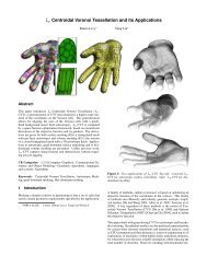
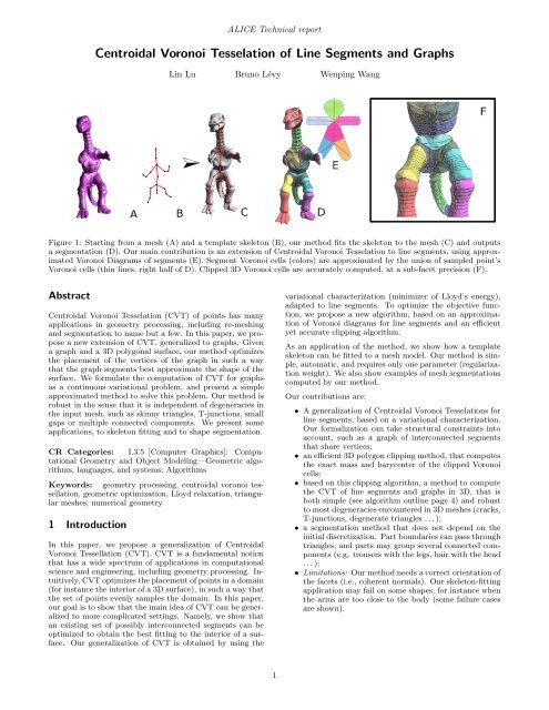
Figure 1: Starting from a mesh (A) and a template skeleton (B), our method fits the skeleton to the mesh (C) and outputs
a segmentation (D). Our main contribution is an extension of Centroidal Voronoi Tesselation to line segments, using approximated
Voronoi Diagrams of segments (E). Segment Voronoi cells (colors) are approximated by the union of sampled point’s
Voronoi cells (thin lines, right half of D). Clipped 3D Voronoi cells are accurately computed, at a sub-facet precision (F).
Abstract
Centroidal Voronoi Tesselation (CVT) of points has many
applications in geometry processing, including re-meshing
and segmentation to name but a few. In this paper, we propose
a new extension of CVT, generalized to graphs. Given
a graph and a 3D polygonal surface, our method optimizes
the placement of the vertices of the graph in such a way
that the graph segments best approximate the shape of the
surface. We formulate the computation of CVT for graphs
as a continuous variational problem, and present a simple
approximated method to solve this problem. Our method is
robust in the sense that it is independent of degeneracies in
the input mesh, such as skinny triangles, T-junctions, small
gaps or multiple connected components. We present some
applications, to skeleton fitting and to shape segmentation.
CR Categories: I.3.5 [Computer Graphics]: Computational
Geometry and Object Modeling—Geometric algorithms,
languages, and systems; Algorithms
Keywords: geometry processing, centroidal voronoi tessellation,
geometric optimization, Lloyd relaxation, triangular
meshes, numerical geometry
1 Introduction
In this paper, we propose a generalization of Centroidal
Voronoi Tessellation (CVT). CVT is a fundamental notion
that has a wide spectrum of applications in computational
science and engineering, including geometry processing. Intuitively,
CVT optimizes the placement of points in a domain
(for instance the interior of a 3D surface), in such a way that
the set of points evenly samples the domain. In this paper,
our goal is to show that the main idea of CVT can be generalized
to more complicated settings. Namely, we show that
an existing set of possibly interconnected segments can be
optimized to obtain the best fitting to the interior of a surface.
Our generalization of CVT is obtained by using the
variational characterization (minimizer of Lloyd’s energy),
adapted to line segments. To optimize the objective function,
we propose a new algorithm, based on an approximation
of Voronoi diagrams for line segments and an efficient
yet accurate clipping algorithm.
As an application of the method, we show how a template
skeleton can be fitted to a mesh model. Our method is simple,
automatic, and requires only one parameter (regularization
weight). We also show examples of mesh segmentations
computed by our method.
Our contributions are:
• A generalization of Centroidal Voronoi Tesselations for
line segments, based on a variational characterization.
Our formalization can take structural constraints into
account, such as a graph of interconnected segments
that share vertices;
• an efficient 3D polygon clipping method, that computes
the exact mass and barycenter of the clipped Voronoi
cells;
• based on this clipping algorithm, a method to compute
the CVT of line segments and graphs in 3D, that is
both simple (see algorithm outline page 4) and robust
to most degeneracies encountered in 3D meshes (cracks,
T-junctions, degenerate triangles . . . );
• a segmentation method that does not depend on the
initial discretization. Part boundaries can pass through
triangles, and parts may group several connected components
(e.g. trousers with the legs, hair with the head
. . . );
• Limitations: Our method needs a correct orientation of
the facets (i.e., coherent normals). Our skeleton-fitting
application may fail on some shapes, for instance when
the arms are too close to the body (some failure cases
are shown).
1

ALICE Technical report
Figure 2: Principle of our method: two examples of Centroidal Voronoi Tesselations for connected line segments in 2D.
2 Previous Work
Centroidal Voronoi Tesselation
CVT for points A complete survey about CVT is beyond
the scope of this paper. The reader is referred to the survey
in [Du et al. 1999]. We will consider here the context of
Geometry Processing, where CVT was successfully applied
to various problems. Alliez et al. developed methods for
surface remeshing [2002], surface approximation [2004] and
volumetric meshing [2005]. Valette et al. [2004; 2008] developed
discrete approximations of CVT on mesh surfaces
and applications to surface remeshing. In all these works,
the nice mathematical formulation of CVT resulted in elegant
algorithms that are both simple and efficient. However,
they use some approximations, that make them dependent
on the quality of the initial mesh. For instance, applications
of these methods to mesh segmentation are constrained to
follow the initial edges, and applications to 3D meshing need
to approximate the clipped Voronoi cells using quadrature
samples.
Recently, the computation of CVT was fully characterized
as a smooth variational problem, and solved with a quasi-
Newton method [Liu et al. 2008]. In this paper, we use the
smooth variational approach, and replace the approximations
used in previous works with an accurate computation
of the clipped 3D Voronoi cells, thus making our algorithm
independent of the initial discretization.
CVT for line segments A first attempt to compute
segment CVT was made in 2D, in the domain of Non-
Photorealistic Rendering [Hiller et al. 2003]. The approach is
based on a heuristic, that is difficult to generalize in 3D, and
that cannot be applied to graphs (more on this below). In
contrast, we propose a variational characterization of CVT
together with a general algorithm to solve the variational
problem.
Skeleton Extraction
Numerous methods have been proposed to extract the skeleton
of a 3D shape. We refer the reader to the survey [Cornea
and Min 2007]. Based on the underlying representation, they
can be classified into two main families :
Discrete volumetric methods resample the interior of
the surface, using for instance voxel grids [Ju et al. 2007;
Wang and Lee 2008]. Baran et al.[2007] construct a discretized
geometric graph and then minimize a penalty function
to penalize differences in the embedded skeleton from
the given skeleton. The advantage of volumetric methods is
that since they resample the object, they are insensitive to
poorly shaped triangles in the initial mesh. However, they
are limited by the discretization and may lack precision, especially
when the mesh has thin features.
Continuous surface methods work on a polygonal mesh
directly. Last year, [Au et al. 2008] proposed a simple skeleton
extraction method based on Laplacian smoothing and
mesh contraction. However, since it relies on a differential
operator on the mesh, it fails to give good results for meshes
with bad quality or with unwanted shape features like spikes,
hair or fur. Methods based on Reeb graph [Aujay et al. 2007]
encounter the same problem. More importantly, they cannot
extract a continuous skeleton from a mesh with multiple connected
components. Methods that extract the skeleton from
a segmentation of the model [Katz and Tal 2003], [Schaefer
and Yuksel 2007],[de Aguiar et al. 2008] suffer from the same
limitation.
In this paper, we propose a volumetric method that directly
uses the initial representation of the surface. At each iteration,
the interior of the surface is represented by a set of
tetrahedra. Therefore our approach shares the advantage of
volumetric methods (robustness) and the advantage of surfacic
ones (accuracy).
3 Centroidal Voronoi Tessellation for line
segments and graphs
We now present our approach to generalize Centroidal
Voronoi Tesselation (CVT) to line segments and graphs.
Such a generalization of CVT to line segments is likely to
have several applications, such as skeleton fitting and segmentation
demonstrated here, and also vector field visualization
or image stylization. The idea is illustrated in Figure 2.
This section is illustrated with 2D examples, but note that
the notions presented here are dimension independent. Our
results in 3D are shown further in the paper. As shown in
Figure 2, starting from an initial configuration of the skeleton,
we minimize in each Voronoi cell (colors) the integral
of the squared distance to the skeleton (generalized Lloyd
energy). This naturally fits the edges of the skeleton into
the protrusions of the mesh.
We first recall the usual definition of CVT for points (Section
3.1), then we extend the definition to line segments and
graphs (Section 3.2), and introduce the approximation that
we are using (Section 3.3). Section 3.4 introduces the regularization
term, and Section 4 our solution mechanism.
3.1 CVT for points
CVT has diverse applications in computational science and
engineering, including geometry processing [Du et al. 1999;
Alliez et al. 2005] and has gained much attention in recent
years. In this paper we extend the definition of CVT to
make it applicable for sets of inter-connected line segments
(or graphs). We first give the usual definition of Voronoi
Diagram and Centroidal Voronoi Tesselation.
2

ALICE Technical report
(a)
(b)
Figure 3: CVT for points in 2D.
Figure 5: Voronoi diagram of two line segments.(a)Accurate
VD; (b)approximated VD.
Let X = (x i) n i=1 be an ordered set of n seeds in R N . The
Voronoi region V or(x i) of x i is defined by :
V or(x i) = {x ∈ R N
| ‖x − x i‖ ≤ ‖x − x j‖, ∀j ≠ i}.
The Voronoi regions of all the seeds form the Voronoi diagram
(VD) of X. Let us now consider a compact region
Ω ⊂ R N (for instance, the interior of the square around Figure
3-left). The clipped Voronoi diagram is defined to be the
set of clipped Voronoi cells {V or(x i) ∩ Ω}.
A Voronoi Diagram is said to be a Centroidal Voronoi Tesselation
(CVT) if each seed x i coincides with the barycenter
of its clipped Voronoi cell (geometric characterization).
An example of CVT is shown in Figure 3-right. This definition
leads to Lloyd’s relaxation [Lloyd 1982], that iteratively
moves all the seeds to the barycenter of their Voronoi cells.
Alternatively, CVT can be also characterized in a variational
way [Du et al. 1999], as the minimizer of Lloyd’s energy F :
F (X) =
nX
Z
f(x i) ; f(x i) =
i=1
V or(x i )∩Ω
‖x−x i‖ 2 dx (1)
Using this latter variational formulation, a possible way of
computing a CVT from an arbitrary configuration consists
in minimizing F [Liu et al. 2008]. Now we explain how this
variational point of view leads to a more natural generalization
to line segments as compared to the geometric characterization
used in Lloyd’s relaxation.
3.2 CVT for line segments and graphs
Besides points, it is well known that general objects such as
line segments can also be taken as the generators of Voronoi
diagrams (see Figure 4). For instance, Hiller et al. [2003]
have used line segments Voronoi diagrams to generalize the
notion of stippling used in Non-Photorealistic Rendering.
Their method uses a discretization on a pixel grid, and a
heuristic based on a variant of Lloyd’s relaxation to move the
segments. They translate each segment to the centroid of its
Voronoi cell, and then align it with the cell’s inertia tensor.
In our case, it is unclear how to apply this method to a set of
segments that share vertices (i.e. a graph). Moreover, using
a pixel grid is prohibitively costly in 3D.
For these two reasons, we consider the variational characterization
of CVT, that we generalize to line segments. Let E
be the set of line segments with the end points in X. We
define the CVT energy for segment [x i, x j] in Ω as:
g([x i, x j]) =
Z
Vor([x i ,x j ]) T Ω
d(z, [x i, x j]) 2 dz, (2)
where Vor([x i, x j]) = {z ∈ R N | d(z, [x i, x j]) ≤ d(z, [x k , x l ]),
∀k, l ∈ E} and d(z, [x i, x j]) denotes the Euclidean distance
from a point to the segment.
Particularly, when the same vertex is shared by several line
segments, they define a graph. We denote this graph by
G := (X, E).
Definition 1 A CVT for a graph G = (X, E) is the minimizer
X of the objective function G defined by :
G(X) = X
g([x i, x j]). (3)
i,j∈E
In practice, minimizing G is non-trivial, due to the following
two difficulties :
• Computing the VD of line segments is complicated,
since the bisector of two segments are curves (resp. surfaces
in 3D) of degree 2. Some readily available software
solve the 2D case (e.g., VRONI [Held 2001] and
CGAL), but the problem is still open in 3D ;
• supposing the VD of line segments is known, integrating
distances over cells bounded by quadrics is non-trivial.
3.3 Approximated CVT for segments and graphs
For these two reasons, we use an approximation. As shown
in Figure 5, we replace the segment [x i, x j] with a set of
samples (p k ) :
p k = λ k x i + (1 − λ k )x j , λ k = [0, 1].
Then the Voronoi cell of the segment can be approximated
by the union of all intermediary points’ Voronoi cells, and
its energy g can be approximated as follows :
Vor([x i, x j]) ≃ [ k
Vor(p k ) ; g([x i, x j]) ≃ X k
f(p k )
Figure 4: CVT for segments in an ellipse.
where f denotes the point-based energy (Equation 1).
This yields the following definition :
3

ALICE Technical report
(a) (b) (c)
Figure 6: A chained graph with 5 vertices and 4
edges.(a)Input; (b)minimizer of CVT energy; (c)with regularization
energy γ = 0.01.
(a)
(b)
Figure 7: (a)γ = 0, 0.01 from left to right; (b) γ = 0, 0.03, 0.1
respectively from left to right.
Definition 2 An Approximate CVT for a graph G = (X, E)
is the minimizer X of the objective function G e defined by :
eG(X) = X X
f(p k ) = X X
f(λ k x i + (1 − λ k )x j).
i,j∈E
k
i,j∈E
where f denotes the point-based energy (Equation 1).
Since it is based on a standard Voronoi diagram and Lloyd
energy, the so-defined approximated objective function e G is
much simpler to optimize than the original G given in Equation
3. Note that G and e G depend on the same variables X.
The intermediary samples p k = λ k x i + (1 − λ k )x j are not
variables, since they depend linearly on x i and x j.
To avoid degenerate minimizers, we now introduce a stiffness
regularization term, similarly to what is done in variational
surface design.
3.4 Regularization, stiffness
The CVT energy tends to maximize the compactness of the
dual Voronoi cells, which is desired in general. However,
some particular configurations may lead to unwanted oscillations.
For instance, the (undesired) configuration shown in
Figure 6(b) has a lower energy than the one shown in Figure
6(c). Intuitively, the long thin cells in (c) have points that
are far away from the skeleton. To avoid the configuration
in (b) and favor the one in (c), we add a regularization term
R(X) to the energy functional, defined as the squared graph
Laplacian, that corresponds to the stiffness of the joints :
R(X) =
X
x i ,v(x i )>1
k
‖x i − 1
v(x i)
X
x j ∈N(x i )
(4)
x j‖ 2 , (5)
where v(x i) denotes the valence, N(x i) the neighbors of x i.
We can now define the objective function F minimized by
our approach :
F(X) = e G(X) + γ|Ω|R(X). (6)
where e G(X) is the approximated Lloyd energy of the segments
(Equation 4) and R(X) is the regularization term
(Equation 5). γ ∈ R + denotes the influence of the regularization
term. We used γ = 0.01 in all our experiments.
Note that the regularization term R is multiplied by the
volume of the object |Ω| so that e G and R have compatible
dimensions.
Figure 7 shows the influence of the parameter γ. For valence
2 nodes, a high value of γ tends to straighten the joints.
For branching nodes, a high value of γ tends to homogenize
the segment angles and lengths. In our experiments,
good results were obtained with γ = 0.02. It is also possible
to assign a different stiffness γ i to each joint, to improve
joint placement, but since this introduces too many parameters,
we will show later a simpler method to automatically
optimize joint placements, without needing any additional
parameter.
4 Solution mechanism
To minimize the objective function F, we use an efficient
quasi-Newton solver. A recent work on the CVT energy
showed its C 2 smoothness [Liu et al. 2008] (except for some
seldom encountered degenerate configurations where it is
C 1 ). In our objective function F, the term ˜G composes
linear interpolation with the Lloyd energy, and the regularization
term R is a quadratic form. Therefore, F is also
of class C 2 , which allows us to use second-order optimization
methods. As such, Newton’s algorithm for minimizing
functions operates as follows :
(1) while ‖∇F(X)‖ > ɛ
(2) solve for d in ∇ 2 F(X)d = −∇F(X)
(3) find a step length α such that
F(X + αd) sufficiently decreases
(4) X ← X + αd
(5) end while
where ∇F(X) and ∇ 2 F(X) denote the gradient of F and its
Hessian respectively. Computing the Hessian (second-order
derivatives) can be time consuming. For this reason, we use
L-BFGS [Liu and Nocedal 1989], a quasi-Newton method
that only needs the gradient (first-order derivatives). The
L-BFGS algorithm has a similar structure, with a main loop
that updates X based on evaluations of F and ∇F. The
difference is that in the linear system of line (2), the Hessian
is replaced with a simpler matrix, obtained by accumulating
successive evaluations of the gradient (see [Liu and Nocedal
1989] and [Liu et al. 2008] for more details).
In practice, one can use one of the readily available implementations
of L-BFGS (e.g. TAO/Petsc).
Thus, to minimize our function F with L-BFGS, what we
need now is to be able to compute F(X) and ∇F(X) for
a series of X iterates, as in the following outline, detailed
below (next three subsections).
4

ALICE Technical report
Figure 8: Illustration of the sampling on the segments.
Algorithm outline - CVT for line segments and graphs
For each Newton iterate X
1. For each segment [x i, x j], generate the samples p k ;
2. For each p k , compute the clipped Voronoi cell of p k ,
i.e. V or(p k ) ∩ Ω where Ω denotes the interior of the
surface ;
3. Add the contribution of each p k to F and ∇F.
4.1 Generate the samples p k
We choose a sampling interval h. In our experiments,
1/100 th of the bounding box’s diagonal gives sufficient precision.
We then insert a sample every h along the segments.
Terminal vertices (of valence 1) are inserted as well.
Vertices x i of valence greater than 1 are skipped, in order to
obtain a good approximation of the bisectors near branching
points (see Figure 8).
4.2 Compute the clipped Voronoi cells
We now compute the Delaunay triangulation of the samples
p k (one may use CGAL for instance), and then the
Voronoi diagram is obtained as the dual of the Delaunay
triangulation. Now we need to compute the intersections
between each Voronoi cell V or(p k ) and the domain Ω, defined
as the interior of a triangulated surface. Since Voronoi
cells are convex (and not necessarily the surface), it is easier
(though equivalent) to consider that we clip the surface by
the Voronoi cell. To do so, we use the classical re-entrant
clipping algorithm [Sutherland and Hodgman 1974], recalled
in Figure 9-A, that considers a convex window as the intersection
of half-spaces applied one-by-one to the clipped
object. In our 3D case, when clipping the triangulated surface
with a half-space, each triangle can be considered independently.
We show an example in Figure 9-B, where two
bisectors generate Homer’s “trousers”. Since it processes
the triangles one by one, the algorithm is extremely simple
to implement, and does not need any combinatorial data
structure. Moreover, it can be applied to a “triangle soup”,
provided that the polygons have correct orientations (i.e.,
coherent normals).
However, it is important to mention that the surface needs
to be closed after each half-space clipping operation. This
is done by connecting each intersection segment (thick red
in Figure 9-C) with the first intersection point, thus forming
a triangle fan. Note that when the intersection line is
non-convex, this may generate geometrically incorrect configurations,
such as the sheet of triangles between the legs
Figure 9: Sutherland-Hogdman re-entrant clipping.
in Figure 9-D. However, this configuration is correct from a
computational point of view, if we keep the orientation of
the triangles, as explained in Figure 9-E. Suppose we want
to compute the area of the “bean” shape, by summing triangles
connected to the red vertex. With the orientation of the
triangles, the extraneous area appears twice, with a positive
and negative orientation that cancel-out. After the clipping
operation, the clipped Voronoi cell of the point p k is represented
by its boundary, as a list of triangles (q i, q j, q k ).
The interior of the Voronoi cell is obtained as a set of oriented
tetrahedra (p k , q i, q j, q k ), created by connecting p k to
each triangle. Note also that p k may be outside its clipped
Voronoi cell, but again, with the orientation of the tetrahedra,
this still gives the correct result for Lloyd’s energy,
barycenter and mass computed in the next section.
4.3 Add the contributions to F and ∇F
We first consider the approximated segment Lloyd energy
eG. The CVT energy associated with a tetrahedron T =
(p k , q 1, q 2, q 3) is given by
|T |
10 (U2 1 + U 2 2 + U 2 3 + U 1.U 2 + U 2.U 3 + U 3.U 1),
where U i = q i − p k and |T | denotes the oriented volume of
T . To compute the gradients, we first recall the gradient of
the point-based Lloyd energy [Du et al. 1999], given by :
∂F
∂p k
= 2m k (p k − c k )
where:
m k =
R
V or(p k )∩Ω
dx ; c k = 1
R
m k
V or(p k )∩Ω
xdx
By applying the chain rule to the expression of the intermediary
points p k = λ k x i + (1 − λ k )x j, we obtain the gradient
(7)
5

ALICE Technical report
Figure 11: Influence of the initialization.
Figure 10: Fitting and segmentation before (top) and after
joint optimization (bottom). Notice the rightmost knee.
of e G for the edge [x i, x j] :
∂ e G
∂x i
= X k
= X k
∂ e G
∂x j
= X k
∂f(p k )
∂x i
∂f(p k ) ∂p k
= 2 X ∂p k ∂x i
k
∂f(p k )
∂x j
= 2 X k
m k (p k − c k )λ k ;
m k (p k − c k )(1 − λ k ),
where m k and c k denote the mass and the centroid of
V or(p k ) ∩ Ω respectively (see Equation 7). Note that m k
and c k can be easily computed from the clipped Voronoi cell,
represented by a union of oriented tetrahedra (see section 4).
The gradient of e G with respect to the graph vertex x i gathers
the contributions of all the gradients of the sampling points
p k in the segments incident to x i.
The contribution of the regularization term to the gradient
∇R is given by :
0
∂R
= 2|Ω|γ i
@x i − 1
∂x i v(x i)
4.4 Optimize joint placement
X
x j ∈N(x i )
x j
1
A .
The objective function F only takes geometry into account,
and does not necessarily places the joints where the user expects
them. For instance, for a straight arm, the joint will
be located at the middle, which does not necessarily corresponds
to the elbow. However, from the information computed
by our algorithm, it is easy to optimize the location of
the joints. Our algorithm computes all the intersections between
the Voronoi cells and the mesh, shown as black lines
in Figure 10. Each black line is associated with a sample
of the skeleton. The elbows correspond to constrictions, i.e.
black lines of minimal length. Therefore, for each joint, we
determine the sample in the neighborhood of the joint that
has an intersection curve of minimal length, and move the
joint to the location of this sample. For each joint x i, we
test the samples in all the bones connected to x i, in the half
of the bone that contains x i.
5 Results and conclusion
We have experimented with our method using several
datasets. For a typical mesh, our method converged in 5
Newton iterations, which takes 2 minutes on a 2.5 GHz machine.
As demonstrated in Figure 11, our method is reasonably
independent of the initial position (A,B), but may fail for
more extreme initially mismatched configurations (C). In
subsequent tests, initialization is provided by aligning the
bounding box of the skeleton, as done in [Baran and Popović
2007]. Our method is robust to mesh degeneracies (Figure
12), such as T-Junctions, and small gaps (red lines), thanks
to the accurate computation of clipped Voronoi cells (thick
black lines) and the triangle-by-triangle (or tet-by-tet) integration.
Figure 13 shows that noisy meshes with skinny
triangles can be processed without any numerical instability
(data acquired by the Visual Hull technique). To our
knowledge, this is the first method that achieves this degree
of robustness.
Figure 14 shows the influence of the edge sampling interval
h, used to approximate the segment Voronoi cells. As can be
seen, a coarse sampling is sufficient to obtain a result similar
to the one obtained with a finer sampling. However, we use
h = 1/100 th of the bounding box diagonal (left), to have
enough samples for the joint placement optimization phase
(Section 4.4).
We show in Figure 15 some examples from the SHREK
database. More examples are shown in Figure 16. Except
for a small number of failure cases (red crosses), satisfying
results were obtained. Our method was successfully applied
to meshes with degeneracies (multiple components, holes,
T-junctions) that cannot be processed by previous work.
In addition, a segmentation is obtained, that can be used
for matching features between meshes and morphing. Our
method failed in some cases. One example of failure is shown
in Figure 15 (red cross), where the arms are close to the body.
Figure 17 compares our method with the method using mesh
contraction [Au et al. 2008]. The Monkey’s hair appear as
singularities in Laplacian computation (A). Our volumetric
method is not affected by these singularities (B). Surfacic
methods cannot generate a connected skeleton for a mesh
with multiple components (C), whereas our volumetric approach
does not “see” the boundaries between them (D).
6

ALICE Technical report
Figure 15: Humen from the SHREK database.
Figure 13: Robustness to mesh degeneracies (flat triangles).
Figure 12: Robustness to mesh degeneracies (small holes).
Figure 14: Influence of the skeleton sampling. With a coarse
sampling of the skeleton (right) one obtains a result similar
to the one obtained with a finer sampling (left).
7

ALICE Technical report
Figure 16: More results of our method.
Conclusion We have presented in this paper a new method
for variational skeleton fitting. Its main advantages are :
• Simplicity: the problem of skeleton fitting is expressed
in variational form (Equation 6), requiring no more
than minimizing an objective function. The gradients
are easily computed by our Voronoi clipping;
• Robustness: the triangle-by-triangle integration (tetby-tet)
does not need a connected mesh, and does not
estimate differential quantities, therefore our method
works with degenerate meshes.
This paper showed results for skeleton fitting and shape segmentation.
We think that other applications are possible,
such as shape morphing, shape retrieval and markerless motion
capture by fitting skeletons to mesh sequences acquired
by computer vision. We showed that generalizing the Centroidal
Voronoi Tesselation framework to primitives that are
more general than points is possible. Beyond the graph of
segments considered here, in future work we will consider
CVT-based shape optimization by defining CVT with other
types of primitives (i.e. cylinders, plates . . . ).
Acknowledgments
References
will be given in the final version.
Alliez, P., Meyer, M., and Desbrun, M. 2002. Interactive Geometry
Remeshing. ACM TOG (Proc. SIGGRAPH) 21(3), 347–354.
Alliez, P., Cohen-Steiner, D., Yvinec, M., and Desbrun, M. 2005.
Variational tetrahedral meshing. ACM TOG (Proc. SIGGRAPH).
Au, O. K.-C., Tai, C.-L., Chu, H.-K., Cohen-Or, D., and Lee, T.-Y.
2008. Skeleton extraction by mesh contraction. ACM TOG (Proc.
SIGGRAPH .
Aujay, G., Hétroy, F., Lazarus, F., and Depraz, C. 2007. Harmonic
skeleton for realistic character animation. In Proc. SCA.
Baran, I., and Popović, J. 2007. Automatic rigging and animation of
3d characters. ACM TOG (Proc. SIGGRAPH .
Cohen-Steiner, D., Alliez, P., and Desbrun, M. 2004. Variational
shape approximation. ACM TOG (Proc. SIGGRAPH).
Cornea, N. D., and Min, P. 2007. Curve-skeleton properties, applications,
and algorithms. IEEE TVCG 13, 3.
Figure 17: Comparison between Au et al.’s mesh-contraction
(left) and our method (right).
de Aguiar, E., Theobalt, C., Thrun, S., and Seidel, H.-P. 2008. Automatic
Conversion of Mesh Animations into Skeleton-based Animations.
Computer Graphics Forum (Proc. Eurographics).
Du, Q., Faber, V., and Gunzburger, M. 1999. Centroidal Voronoi
tessellations: applications and algorithms. SIAM Review.
Held, M. 2001. VRONI: An engineering approach to the reliable
and efficient computation of voronoi diagrams of points and line
segments. Computational Geometry: Theory and Applications.
Hiller, S., Hellwig, H., and Deussen, O. 2003. Beyond stipplingmethods
for distributing objects on the plane. Computer Graphics
Forum.
Ju, T., Baker, M. L., and Chiu, W. 2007. Computing a family of
skeletons of volumetric models for shape description. CAD.
Katz, S., and Tal, A. 2003. Hierarchical mesh decomposition using
fuzzy clustering and cuts. ACM TOG.
Liu, D. C., and Nocedal, J. 1989. On the limited memory BFGS
method for large scale optimization. Mathematical Programming:
Series A and B 45, 3, 503–528.
Liu, Y., Wang, W., Lévy, B., Sun, F., Yan, D. M., Lu, L., and Yang, C.
2008. On centroidal voronoi tessellation - energy smoothness and
fast compu tation. Tech. rep., Hong-Kong University and INRIA -
ALICE Project Team. Accepted pending revisions.
Lloyd, S. P. 1982. Least squares quantization in PCM. IEEE Transactions
on Information Theory 28, 2, 129–137.
Schaefer, S., and Yuksel, C. 2007. Example-based skeleton extraction.
In Proc. SGP.
Sutherland, I. E., and Hodgman, G. W. 1974. Reentrant polygon
clipping. Comm. ACM 17, 1, 32–42.
Valette, S., and Chassery, J.-M. 2004. Approximated centroidal
Voronoi diagrams for uniform polygonal mesh coarsening. Computer
Graphics Forum (Proc. Eurographics).
Valette, S., Chassery, J.-M., and Prost, R. 2008. Generic remeshing
of 3D triangular meshes with metric-dependent discrete Voronoi
diagrams. IEEE TVCG.
Wang, Y.-S., and Lee, T.-Y. 2008. Curve-skeleton extraction using
iterative least squares optimization. IEEE TVCG.
8