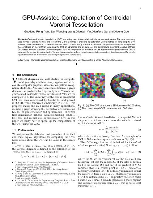
GPU-Assisted Computation of Centroidal Voronoi ... - alice - Loria

3parallel, similar to the flood-filling algorithm, but withfaster speed due to its use of varying step lengths. Wewill use the JFA to compute the Voronoi diagram in2D as well as on a surface. Like [19], [21] we use theEuclidean distance to approximate the geodesic distanceon a surface.To compute the Voronoi diagram on a surface, onemay compute a 3D Voronoi diagram and find its intersectionwith the surface. The GPU has also been usedto compute 3D Voronoi diagrams [27], [30], [31], [32],[33]. Weber et al. [34] adopted the raster scan methodin the geometry image to compute the Voronoi diagramusing the geodesic distance on a surface. This methodhandles disk-like open surfaces only. The geodesic distance,though more accurate than the Euclidean distance,is much less efficient to compute on a mesh surface, evenwith GPU acceleration.Vasconcelos et al.’s work [35] is the only known successfulattempt so far using the GPU to compute the CVTin a plane. They implemented the Lloyd’s method on theGPU to compute the CVT on a 2D plane, focusing on thecomputation of the centroids. A predefined mask is usedto conservatively estimate the Voronoi cell for every site.Since the diameter of a Voronoi cell may be very big, toensure an accurate result, the mask must be as big as thewhole texture, which makes the method inefficient.In contrast, we use the vertex program to performscattering and use the framebuffer blending function toaccumulate the coordinates. Our approach is simpler andworks well for computing both the CVT on a 2D planeand the CCVT on a surface.3 CVT ON 2D PLANEThere are two main steps in both Lloyd’s algorithmand the L-BFGS algorithm: 1) computing the Voronoidiagram of the current sites, and 2) finding new positionsof the sites for the next iteration. For step 1, we computea discrete approximation of the Voronoi diagram usingthe jump flooding algorithm (JFA) [22] on the GPU. Wepropose a new regional reduction method for efficientlycomputing various integrals needed in step 2. In thefollowing we will briefly review the JFA and present theregional reduction technique.3.1 Jump Flooding AlgorithmSuppose that there is a site in an n × n texture in theGPU and we want to propagate some information (e.g.the coordinates of the site) from the site to all the otherpixels. The JFA performs this in several passes. For aninitial step length k that is a power of 2 (e.g. 2 ⌈log n⌉ ),a pixel at (x, y) passes its information to its neighbors(eight at most) at (x + i, y + j), where i, j ∈ {−k, 0, k}(Fig. 2). Then in the subsequent passes, the same propagationis performed for a pixel using the step lengththat is half of the previous step length k. The iteration isstopped when the step length reaches 1. Fig. 2 illustratesk=4 k=2 k=1Fig. 2. The iterations of the JFA for an 8×8 texture withan initial site at the bottom left corner.how the JFA fills up an 8×8 texture using three passeswith the single initial site at the bottom left corner.When using the JFA to compute the Voronoi diagramin a 2D texture, there are multiple sites and the informationto be propagated from each site is its coordinates.Upon receiving the coordinates of different sites, eachpixel compares its distances to these sites to find thenearest site whose Voronoi cell it belongs to. Thus allthe pixels are classified to form a Voronoi diagram.Despite its fast speed, the JFA may misclassify a smallnumber of pixels [22]. We use 1+JFA [33], an improvedversion of JFA, to compute the Voronoi diagram in ourGPU implementations. On average, the error rate of1+JFA is less than 0.25 pixels in a texture with theresolution of 512×512 for less than 10,000 sites, which isaccurate enough for most practical graphics applicationsutilizing the CVT. To be brief, we will refer 1+JFA as JFAas well.A sufficiently large initial step length is needed toensure that each pixel is reached by its nearest site.On the other hand, one should try to use a small but“safe” initial step length to reduce the computation timeincurred by unnecessary JFA passes. A safe choice is2 ⌈log n⌉ , which is necessary for computing a Voronoidiagram when the sites are distributed in such a waythat each Voronoi cell is narrow and long, as the cellsgenerated by a sequence of collinear sites. However, thisinitial step length is, overall, very conservative becauseafter a few iterations of CVT computation (with eitherLloyd’s algorithm or the L-BFGS algorithm) the sites arenormally already distributed rather evenly, therefore amuch smaller initial step length would be sufficient foreach pixel to be reached by its nearest site.This consideration leads us to use the followingscheme for selecting the initial step length. In the VDcomputation of the first CVT iteration, the initial steplength of the JFA is set to be 2 ⌈log n⌉ . For the VDcomputation in the next m CVT iterations, we computethe average distance from each site to all the pixelsin its Voronoi cell using the regional reduction (to beintroduced in next subsection), and set the initial steplength of the JFA to be the double of the maximumof all these average distances. Our experiments showthat m = 5 gives satisfactory performance. Then in theremaining CVT iterations (i.e. after 5 iterations) the initialstep length of the JFA is set to be that used in the 5thiteration.

4VC0VC1C1part of Voronoi diagramx00x11x2 x3 x4 ...bottom left part of result textureFig. 3. Illustration of regional reduction. All the pointsin the Voronoi cell i (VC i ) are translated to the pixelcorresponding to the site x i .3.2 Regional ReductionSeveral different integrals over the Voronoi cells of allthe sites need to be evaluated in CVT computation,that is, for computing the value of the CVT energyfunction or computing the centroid as needed by theLloyd algorithm. To approximate these integrals, weneed to perform summations over the pixels of all theVoronoi cells in parallel, which calls for solving the socalledregional reduction problem.In the reduction problem, one needs to reduce a numberof values to a single one, such as sum, maximum,minimum, etc. More precisely, the reduction problemtakes as input a set of values v 1 , . . . , v n and outputs asingle value v = v 1 ⊕ . . . ⊕ v n , where ⊕ is an associativeand commutative operator. Thus, summation is a specialcase of the reduction problem.The reduction problem can be solved in O(log n)passes on the GPU using a fragment program [36].Existing algorithms can only perform global reductions,that is, reducing values of all the pixels in a textureinto one single value. However, in CVT computationthe domain Ω is decomposed into multiple regions (thatis, Voronoi cells) Ω i and we need to compute the sumsof values of the pixels of different regions in parallel.Therefore, we face a regional reduction problem ratherthan a global one.We propose to use the method of rendering pointsfor regional reduction. A single point is rendered forevery pixel, and its position is changed in the vertexprogram. All the points in the Voronoi cell of site x iare translated to the same position decided by its IDi. For example, the site x i corresponds to the position(i/w, i%w), where w is the width of the texture usedand “/” and “%” are division and modulus operators forintegers, respectively. The result is a texture containingthe reduction values for all the Voronoi cells, one pixelfor each site, which are packed in the order of the site’sID. Fig. 3 shows an illustration of this operation.First, every point is rasterized into one fragment.The fragment program processing these fragments thenwrites the values to a texture recording the results. Thedepth test or framebuffer blending operations can beused to reduce all the values corresponding to the samepixel to a single value which is stored in a result texture.For example, if we want to compute the maximum of thevalues, we can write the values into the depth channelas well as the color channels for every fragment, andset the depth test function so that only the fragmentwith the maximum value is stored into the result texture(e.g. using glDepthFunc(GL_GREATER)). If we wantto compute the sum of the values, we can write thevalues into color channels for every fragment, and set theblending function so that the values of all the fragmentsare added and the result is stored into the result texture(e.g. using glBlendFunc(GL_ONE, GL_ONE)).Our regional reduction method works for a connectedregion as well as a set consisting of disconnected regions.This is important because the Voronoi diagram of asurface may contain disconnected Voronoi cells nearthe boundaries of the geometry image (see Section 4).Furthermore, a Voronoi cell in a pixel plane may containdisconnected parts [37]; such a case can be handledproperly by our regional reduction method.3.3 Lloyd’s Algorithm in 2DEvery iteration in Lloyd’s algorithm contains two steps:1) computing the Voronoi diagram of the current sites;and 2) computing the centroids for Voronoi cells as thenew sites in the next iteration. These two steps areiterated until certain termination condition is met.On a 2D plane the centroids are computed using(1). Using regional reduction the integrations in (1) areapproximated by summations, so we have∑∑x∈Ωc i = iρ(x)x∆σ∑x∈Ω iρ(x)∆σ = x∈Ω iρ(x)x∑x∈Ω iρ(x) , (4)where the x is the pixel position and ∆σ the constantarea occupied by each pixel.The numerator and denominator in (4) are computedusing the regional reduction in the same pass since theyshare the same domain. The numerator is a 2D vectorstored in red and green channels of the texture, and thedenominator is a scalar value stored in the blue channel.We stress that the coordinates of each site of theVoronoi diagram are floating point numbers, albeit theyare stored in the discrete pixel closest to it. Since theVoronoi cells are composed of pixels, the Voronoi boundarieshave only pixel precision. The algorithm will stopwhen the Voronoi diagram does not change. Alternatively,a different termination condition can be used bychecking if the value of CVT energy function F or itsgradient has reached a threshold.3.4 L-BFGS Algorithm in 2DThe L-BFGS algorithm is a quasi-Newton algorithm thatis more efficient than Lloyd’s method for CVT computation[21]. In every iteration of the L-BFGS algorithm,we need to compute the CVT energy F and its partialderivatives with respect to all the sites. These valuesare accumulated with those values of the m precedingiterations to approximate the inverse Hessian matrix.

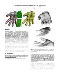
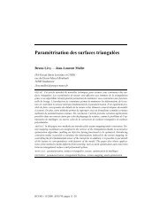
5SufaceParameter DomainInput Data Distortion Factor Initial Sites Initial Voronoi Diagram Final Sites Final CVDFig. 4. The pipeline for computing a CCVT on a surface. From left to right: the input David Head model together withits geometry image ((r,g,b)=(x,y,z)) and normal vector image ((r,g,b)=(n x , n y , n z )), distortion factors (modulated forvisual clarity), the initial sites and the corresponding Voronoi diagram, and the final sites with the CCVT. The top rowshows the parameter domain, and bottom row shows the surface.More specifically, define s k = X k − X k−1 and y k =∇F k − ∇F k−1 , where X k and ∇F k are the ordered set ofsites and the gradient of the CVT energy function F atthe k-th iteration, respectively. Then the approximatedinverse Hessian matrix H k is updated byH k = V T k H k−1V k + ρ k s k s T k (5)where ρ k = 1/yk Ts k, and V k = I −ρ k y k s T k . The new sitesX k+1 for the next iteration is given by X k+1 = X k −H k ∇F k . More details of the L-BFGS algorithm are givenin [21].The first-order partial derivative of F with respect tothe site x i is [2]:∂F∂x i= 2∫Ω iρ(x)(x i − x)dσ. (6)This integral is approximated by summation in the GPUusing the regional reduction, performed in the same passas computing the energy function F . These values arewritten into a texture and read back to the CPU, wherethey are used to compute the approximated inverseHessian matrix H k using (5) and then the new sitesX k+1 . Hence, our implementation of the L-BFGS methodis not entirely done on GPU.4 CCVT ON SURFACESIn this section we will explain the pipeline of computingthe CCVT on a surface, following the flow in Fig. 4.4.1 Geometry Image for Surface RepresentationFor a given surface we first compute a conformal parameterization[38] of the surface over a 2D rectangular domainand use the parameterization to construct a regularquad mesh to represent the surface. Then the surfacecan be represented by a 2D texture called the geometryimage [39] whose pixels store the 3D coordinates of the(a)Fig. 5. (a) A regular triangulation in a geometry image.(b) The corresponding triangulation on the surface.corresponding mesh vertices. The red, green and bluechannels of a geometry image store the 3D coordinatesof the mesh vertices, respectively. The surface normalvectors at the vertices are also stored in a 2D texture ofthe same size, called normal vector image, which will beused in the L-BFGS algorithm for computing the CCVTon a surface.Due to parameterization distortion, each pixel is assigneda weight equal to the area it covers on thesurface. This weight is computed as follows. Supposethat the grid is subdivided to give a regular triangulationas shown in Fig. 5. Every pixel is supposed to coverone-third of each triangle incident to the correspondingvertex of the pixel. Thus the weight of the pixel is setto the 1/3 of the areas of all the triangles incident tothe corresponding vertex. The weight will be called thedistortion factor.The pipeline of computing the CCVT is shown inFig. 4. The left most part of Fig. 4 shows the geometryimage and the normal vector image of the surface ofDavid Head in the top row, and the surface itself and acheckerboard texture showing the parameterization inthe bottom row. The computed distortion factors areshown in the left middle part of Fig. 4.Like the 2D case, computing the CCVT on a surface(b)

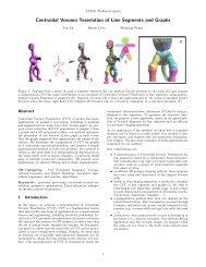
6implement Lloyd’s algorithm and the L-BFGS algorithmon the GPU to compute the CCVT on a surface.(a)Fig. 6. (a) The Voronoi diagram on a surface. (b) Thepartition of the geometry image induced by the Voronoidiagram in (a). The disconnected parts of a Voronoi regionare marked by ellipses in the geometry image.using either Lloyd’s algorithm or the L-BFGS algorithmtakes two main steps in each iteration: 1) computing theVoronoi diagram of the current sites on the surface, and2) computing the new sites for the next iteration. We willexplain these two steps in the following subsections.(b)4.2 Computing Voronoi Diagram on SurfacesSuppose that a given surface is represented as a geometryimage. We first store the 3D coordinates of the initialsites in the nearest corresponding pixels of the geometryimage, and then perform the JFA to compute a Voronoidiagram on the surface. Note that the Euclidean distancebetween points in 3D space is used as approximationto the geodesic distance when computing the Voronoidiagram on the surface.We use a single geometry image for parameterizing asurface of arbitrary topology, with necessary topologicalcutting to facilitate parameterization. Although only surfaceswith simple topology (open surface, cylinder andtorus) can be represented by a geometry image withoutsingularity. The singular points arising from a surfaceof complex topology do not pose any difficulty to ourGPU programs. This is because the JFA only uses the3D coordinates in the Voronoi diagram computation,and does not use the texture coordinates, which are notunique for singular points.Due to topological cut, a Voronoi region on a surfacemay be split into disconnected regions in the geometryimage, as shown by the example in Fig. 6. Here, forexample, because the surface under consideration has acylinder topology, we need to identify the two oppositeboundaries of the geometry image when running the JFAto ensure that a correct Voronoi diagram is computedon the surface. Two disconnected parts in the geometryimage of a connected Voronoi region on the surfaceare marked by ellipses in Fig. 6(b). In this case wecompute the Voronoi diagram by identifying boundariesproduced by topological cut; the result for this exampleis shown in Fig. 6(a).Equipped with the above routine for computing theVoronoi diagram on a surface, we now explain how to4.3 Lloyd’s Algorithm on SurfacesUsing the geometry image to compute the CCVT on asurface with Lloyd’s algorithm follows the same procedureas for computing the CVT in 2D, except that weneed to compute the constrained centroids using (3).The following property about the constrained centroidwill be useful [19]: if c i and c ∗ i are the centroid and theconstrained centroid of the Voronoi cell Ω i respectively,then c i c ∗ i is parallel to the surface normal vector at c ∗ i .On the other hand, we observe that if c ′ i is the nearestpoint in Ω i to c i and it is not on the boundary of Ω i , thenc i c ′ i is parallel to the surface normal vector at c′ i . Basedon these observations we find it an effective heuristicto use the nearest point c ′ i as the constrained centroidc ∗ i in Lloyd’s algorithm, although they are not alwaysidentical, since c i c ′ i being parallel to the surface normalvector at c ′ i is not a sufficient condition for c′ i to be theconstrained centroid.The nearest point c ′ i is computed as follows. For thecorresponding mesh vertex of every pixel in Ω i , we computethe nearest point within its six incident trianglesto the centroid c i . To avoid redundant computations,we only need to check two incident triangles for everyvertex (e.g. the two shaded triangles in Fig. 5 for thecenter vertex), and the other four incident triangles willbe dealt by other neighboring vertices. In this way wefind a nearest point to the centroid c i for every pixel inΩ i . Then by computing the minimum of the distancesfrom these points to c i using the regional reduction, wefind the nearest point c ′ i within Ω i to c i .The number of iterations needed by both Lloyd’s andthe L-BFGS algorithms to obtain the CVT can be reducedsignificantly if the initial sites are roughly evenlydistributed on the surface. To obtain such initial sites,we use the distortion factors as a probability densityfunction to sample the initial sites in the geometry image.Therefore, a pixel with a larger distortion factor is morelikely to be selected as the initial site. The right middlepart of Fig. 4 shows 1,000 initial sites sampled accordingto the distortion factors and the Voronoi diagram generatedin the parameter domain (top row), as well as onthe surface (bottom row). The final sites and the CCVTare shown in the right most part of Fig. 4.4.4 L-BFGS Algorithm on SurfacesThe initial sites for the L-BFGS algorithm are also sampledaccording to distortion factors. In every iteration,to update the sites we need to evaluate the CVT energyfunction F and its partial derivatives. Because the sitesare constrained to be on the surface, we only use thetangential components of the partial derivatives as∂F∂x i∣ ∣∣∣Ω= ∂F∂x i−( ∂F∂x i· N(x i ))N(x i ), (7)

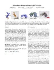
7(a) (b) (c)Fig. 7. The Voronoi diagram of 1,000 initial sites in the 2Ddomain of [−1, 1] × [−1, 1] (a), and CVT results generatedby the L-BFGS algorithm using (b) GPU and (c) CPU.(Unshaded cells are hexagons.)(a)(b)where N(x i ) is the surface normal vector at x i stored inthe normal vector image. Therefore we can use shadersto evaluate F and its partial derivatives on the GPUefficiently, in the same way as in the 2D case.The updated sites computed in the L-BFGS algorithmmay not lie exactly on the surface. We compute theirnearest points in their respective Voronoi cells on thesurface as the new sites on the surface.5 EXPERIMENTAL RESULTS AND DISCUSSIONWe implement our programs using Microsoft VisualC++.net 2005 and NVIDIA Cg 2.0. The hardware platformis Intel Core 2 Duo 2.93GHz with 2GB DDR2RAM, and NVIDIA GeForce GTX 280 with 1GB DDR3VRAM. For the L-BFGS algorithm, we use our HLBFGSlibrary [40]. We have compared our results with the CPUversion of Lloyd’s algorithm and the CPU version ofthe L-BFGS algorithm in [21]. We use m = 7 for allL-BFGS algorithms in our experiments; that is, we usethe gradients of the 7 previous iterations to estimate theinverse Hessian in our implementation.All the programs in this paper use IEEE standard floatpoint numbers (32-bit).5.1 Results of CVT in 2DThe first test example is the computation of the CVTin the 2D domain of [−1, 1] × [−1, 1] mapped to a512×512 texture, with 1,000 random initial sites. TheCVTs computed by the GPU program and CPU programare shown in Fig 7. It is clear that the uniformity ofthe sites is greatly improved in both results. We plotthe CVT energy values and their gradients versus thenumber of iterations for Lloyd’s algorithm and the L-BFGS algorithm in Fig. 8. The red and green curves arefor our GPU programs and the black and blue curvesfor CPU ones. For clarity, we show zoom-in views ofthe shaded regions in Fig. 8(b) and Fig. 8(d).The experiments show that the GPU result is veryclose to the CPU one, although there are fewer hexagoncells in the GPU result and the the final CVT energyvalue generated by the GPU is slightly higher. We may(c)Fig. 8. Energy values (a) and their gradients (c) of CPUand GPU programs for Lloyd’s algorithm and the L-BFGSalgorithm using 1,000 sites in the 2D domain of [−1, 1] ×[−1, 1]. (b) and (d) are zoom-in views of shaded regionsin (a) and (c).evaluate the quality of an approximate CVT by consideringits relative difference from CVT computed with theCPU, defined asCV T energy − final energy CPUfinal energy CPU(d)× 100%,where CV T energy is the CVT energy of the approximateCVT. For the tests shown in Fig. 8 the relativedifference is 0.69% for the result of Lloyd’s algorithmon GPU and 0.58% for that of the L-BFGS algorithm onGPU. These differences can be attributed to two factors.First, a different local minimum with higher energy isproduced by the GPU program. Second, the quantizationerrors in the GPU implementation are responsible.Table 1 compares the total running times of differentprograms for this example. The GPU program and CPUprogram of the same algorithm use the same numberof iterations. Because of the line search used in the L-BFGS minimizer, the function evaluating gradients andenergy value may be called more than once in everyiteration. Within every function call, we need to rebuildthe Voronoi diagram and compute the gradients of theCVT energy, and this is the most time-consuming part ofthe L-BFGS algorithm and dominates the running time.For this reason, #Iter. for the L-BFGS method in Table 1is the number of the function calls.We see that the GPU program of Lloyd’s method isseveral time faster than the CPU program, because all thecomputations for Lloyd’s algorithm are executed on theGPU. However, the GPU program of the L-BFGS methodhas only about 30% speedup over its CPU counterpart.That is because, although the most time-consuming partsfor the L-BFGS algorithm are executed on the GPU, someof its computations are done on the CPU which takesabout 23% of the total time and is not accelerated by the

8TABLE 1Comparison of energy F and running time (in seconds)of different programs using 1,000 initial sites in the 2Ddomain of [−1, 1] × [−1, 1].TABLE 2Comparison of energy F and running time (in seconds)of different programs using 1,000 initial sites in the 2Ddomain of [−1, 1] × [−1, 1] with non-constant densities.Program#Iter.GPUCPUF Time F TimeProgram#Iter.GPUCPUF Time F TimeLloyd 216 2.628×10 3 0.550 2.610×10 3 1.535L-BFGS 92 2.612×10 3 0.512 2.597×10 3 0.703Lloyd 627 6.524×10 −5 2.529 6.163×10 −5 28.530L-BFGS 376 6.185×10 −5 2.301 6.116×10 −5 16.889TABLE 3Information of the five models used in this paper. Thelast two columns are for the number of boundaries andthe resolution of geometry images.Model #Vertices #Faces Genus #B GI(a)Fig. 9. CVT results of 1,000 initial sites generated bythe L-BFGS algorithm in the 2D domain of [−1, 1] ×[−1, 1] with the density function ρ(x) = e −20x2 −20y 2 +0.05 sin 2 (πx)sin 2 (πy) using (a) GPU and (b) CPU.GPU; and the communication between the CPU and theGPU also takes about 5% of the total time.We have also compared our GPU program of Lloyd’smethod to the algorithm proposed by Vasconcelos etal. [35]. For 1,000 sites, even with a very small mask(32×32), their program needs 1.416 seconds for the samenumber of iterations as in Table 1. If the size of themask is set to be same as the screen resolution (512),the running time becomes 44.521 seconds.Our GPU programs can also compute the CVT witha non-constant density function, as the density can besampled and stored as floating point numbers in atexture. An example is shown in Fig 9, comparing theCVTs computed by the GPU program and the CPUprogram of the L-BFGS method. The final CVT energyvalues and the total running time are listed in Table 2.5.2 Results of CCVT on SurfacesWe will compare our GPU programs and CPU programsof Lloyd’s algorithm and the L-BFGS algorithm usingfive surface models: Torus (Fig. 1), Lion (Fig. 10), Sculpture(Fig. 11), Body (Fig. 6), and David Head (Fig. 4).Table 3 lists information about these five models. Allof our experiments use 1,000 initial sites on the surfacesampled according to distortion factors. For each model,the same set of initial sites are used as input for allprograms. The CPU programs utilize the fast algorithmintroduced in [41] which can greatly accelerate the computationof the intersection between the surface andthe 3D Voronoi diagram. For every model the geometryimage is pre-computed with user interaction in less than(b)Torus 4,096 7,938 1 0 512×512Lion 5,321 10,200 0 0 512×190Sculpture 5,471 10,364 3 0 512×372Body 13,978 27,295 0 2 512×456David Head 51,038 101,144 0 1 512×41610 seconds. This time is not included in the total runningtime reported below.The final energy values F and the total running timeof the entire iteration procedure are listed in Table 4 andTable 5. Like the 2D cases, for the L-BFGS algorithm,the number of the function calls for VD computation islisted, rather than the number of iterations. The GPUprogram and the CPU program have the same numberof iterations for Lloyd’s algorithm or the same numberof function calls for the L-BFGS algorithm.It is observed that the GPU programs perform aboutone order of magnitude faster than their CPU counterparts.This speedup is more than that of the 2D casebecause the CPU programs for computing the CCVT of asurface need to compute a 3D Voronoi diagram and findits intersection with the surface, which is a very timeconsuming task compared with computing a Voronoidiagram in a 2D domain. Although the GPU programsalso compute distances in 3D, the whole algorithms arestill efficiently performed in a 2D domain.The relative differences between the GPU and CPUresults range from 0.88% to 8.36% due to differentdistortions of surface parameterizations. Fig. 10 andFig. 11 show two sets of results with the largest relativedifferences of Lion (genus 0) and Sculpture (genus3): the Voronoi diagram of the initial sites, and theCCVTs generated using the GPU and the CPU of Lloyd’salgorithm and the L-BFGS algorithm, with the samenumber of iterations for each algorithm. We note that theGPU results have larger energy values than their CPUcounterparts due its approximation nature.In addition to the comparison in terms of visualinspection and energy values, we may also measure thegeometric uniformity of the sites and their Voronoi cells

9(a) (b) (c) (d) (e)Fig. 10. Comparison of (a) the Voronoi diagram of initial sites and (b-e) the CCVT results on the surface of Lion.Results in (b-e) are generated by Lloyd’s (GPU), L-BFGS (GPU), Lloyd’s (CPU) and L-BFGS (CPU) algorithms,respectively. The relative difference is 5.07% for Lloyd’s algorithm ((b) and (d)) and 6.17% for the L-BFGS algorithm((c) and (e)). As a reference, the CVT energy of the initial sites is 2.538 ×10 −2 , and the relative difference between theinitial sites and the CPU results are 82.85% for Lloyd’s algorithm and 83.12% for the L-BFGS algorithm.(a) (b) (c) (d) (e)Fig. 11. Comparison of (a) the Voronoi diagram of initial sites and (b-e) the CCVT results on the surface of Sculpture.The results in (b-e) are generated by Lloyd’s (GPU), L-BFGS (GPU), Lloyd’s (CPU) and L-BFGS (CPU) algorithms,respectively. The relative difference is 7.88% for Lloyd’s algorithm ((b) and (d)) and 8.36% for the L-BFGS algorithm((c) and (e)). As a comparison, the CVT energy of the initial sites is 8.726 × 10 −3 , and the relative difference betweenthe initial sites and the CPU results are 91.02% for Lloyd’s algorithm and 90.44% for the L-BFGS algorithm.TABLE 4Comparison of energy F and running time (in seconds)of GPU and CPU programs for Lloyd’s algorithm.TABLE 5Comparison of energy F and running time (in seconds)of GPU and CPU programs for the L-BFGS algorithm.Model#Iter.GPUCPUF Time F TimeModel#Iter.GPUCPUF Time F TimeTorus 500 6.381×10 −4 8.235 6.304×10 −4 81.594Lion 135 1.458×10 −2 0.918 1.388×10 −2 20.25Sculpture 183 4.928×10 −3 2.229 4.568×10 −3 27.86Body 262 1.801×10 −4 3.760 1.776×10 −4 52.985David Head 215 9.998×10 −4 2.937 9.839×10 −4 144.688Torus 47 6.362×10 −4 0.808 6.307×10 −4 7.531Lion 28 1.472×10 −2 0.207 1.386×10 −2 3.500Sculpture 26 4.965×10 −3 0.331 4.582×10 −3 3.329Body 67 1.790×10 −4 1.004 1.774×10 −4 13.703David Head 33 1.010×10 −3 0.456 9.854×10 −4 15.609in the CCVT results. For every site x i , we define theradius r i of its Voronoi cell Ω i , the distance d i to itsnearest neighboring site, and the area a i of its Voronoicell Ω i as follows:r i = maxx∈Ω i||x − x i ||, d i = minj≠i ||x i − x j ||, a i = Area(Ω i ).The standard deviations of r i , d i , and a i are used tomeasure the uniformity of a set of sites. Table 6 lists thestandard deviations for initial sites and the sites in theCCVT results on Lion. The uniformity of the initial sitesis greatly improved in all the results. Again, the GPUresults are overall still not as good as the CPU ones.

10TABLE 6Comparison of the uniformity of 1,000 initial sites and thesites in CCVT results generated by different programs onthe surface of Lion.Program STDEV(r i ) STDEV(d i ) STDEV(a i )Initial Sites 1.450×10 −2 1.809×10 −2 3.717×10 −3Lloyd - GPU 7.422×10 −3 9.246×10 −3 1.902×10 −3Lloyd - CPU 3.228×10 −3 6.090×10 −3 1.002×10 −3L-BFGS - GPU 6.992×10 −3 9.657×10 −3 1.805×10 −3L-BFGS - CPU 2.868×10 −3 5.824×10 −3 9.046×10 −4(a)(b)The quality of the CCVT we computed with the GPUis heavily affected by the distortion factors. If the distortionfactors are very large in a certain part of a surface,the Voronoi cells in this part are mapped to a very smallregion in the geometry image. Then the resolution ofthe geometry image will not be adequate for accuratecomputation in this part of the surface, resulting in largererrors in the computation of centroids (for Lloyd’s algorithm)or energy value and gradients (for the L-BFGSalgorithm). To illustrate this, we compare the resultson David Head using two different parameterizations(see Fig. 12). Clearly, the second parameterization haslarger distortion, which leads to more artifacts than thefirst parameterization. This problem could be alleviatedby using a geometry image of higher resolution (seethe example in Fig. 12(e) and (h)), or using multiplegeometry images based a multi-chart surface parameterization[42].The CCVT can be used for surface remeshing bycomputing a well-shaped triangulation of the surface asthe dual mesh of a CCVT. Fig. 13 shows an example ofremeshing the Body surface with 1,000 sites.(c) (d) (e)(f) (g) (h)Fig. 12. (a)&(b) Comparison of two different parameterizationsof David Head. (c) the CVTs computed using theparameterization in (a) with a 512×416 geometry image;(d) the CVTs computed using the parameterization in (b)with a 512×191 geometry image; and (e) the CVTs computedusing the parameterization in (b) with a 2048×765geometry image. (f)-(h) are enlarged top views of thecircled part.5.3 JFA ErrorsIdeally, the CVT energy should decrease monotonicallyduring the iterations in both Lloyd’s and the L-BFGSalgorithm, if implemented accurately. However, sincesome pixels may be misclassified by the JFA into otherVoronoi cells, the partial CVT energy values computedfor those Voronoi cells are slightly different to the accuratevalues. Despite this, the sites move greatly and thetotal CVT energy keeps decreasing in early iterations.However, in late iterations, when most of sites are nolonger moving, the error of JFA may cause the CVTenergy to fluctuate. When this happens, most sites wouldremain unchanged but a small number of sites mayoscillate between some positions.To evaluate the consequence of this oscillation, wecompared the JFA with an implementation on the GPUwhich computes the distance from every pixel to everysite accurately by brute force, and show the results inFig. 14. We see that the energy values only begins tooscillate in very late iterations due to the errors of theJFA.(a)Fig. 13. (a) The dual triangle mesh of 1,000 initial sites;and (b) dual triangle mesh of 1,000 final sites of the CCVT.The insets show the corresponding Voronoi diagrams onthe surface.(b)

11TABLE 8Comparison of Cg and CUDA running time (in seconds)of the L-BFGS algorithm for 1,000 sites in the 2D domainof [−1, 1] × [−1, 1]. All steps are executed 92 times.(a)Fig. 14. Energy values of Lloyd’s algorithm using the JFAand an accurate method to compute the Voronoi diagramof 1,000 sites on Sculpture. (b) A zoom-in view of energyplots in the shaded region in (a).TABLE 7Comparison of Cg and CUDA running time (in seconds)of Lloyd’s algorithm for 1,000 sites in the 2D domain of[−1, 1] × [−1, 1]. All steps are executed 243 times.(b)Step Cg Time CUDA TimeJFA 0.637 0.775Compute Centroids 0.237 0.413Test Stop Condition 0.015 0.107Draw New Sites 0.041 0.032Total Time 0.931 1.327In practice, this oscillation is very small and so doesnot affect the quality of the CVT for most applications ingraphics. One may handle this nonconvergent behaviorby terminating the computation when the CVT energyis found to increase.5.4 Shader Language VS. CUDACUDA is a relatively new and popular C-like languagefor general purpose computation on the GPU. SinceCUDA has some features not available in traditionalshader languages (such as accessing the shared memory),it is much faster for applications which can benefitfrom the new features. However, Cg is better suited thanCUDA for implementing CVT algorithms. To compareCg and CUDA programs, we list detailed time breakdownfor each step in Lloyd’s algorithm and the L-BFGSalgorithm for a 2D case in Table 7 and Table 8 (the timeis the total time for all iterations). It is clear that theJFA and the regional reduction (computing centroid forLloyd’s algorithm, and computing CVT energy and itsgradient for the L-BFGS algorithm) are the two stepsdominating the total running time. The Cg version isfaster for both steps than the CUDA version. In total,the CUDA versions are more than 40% slower than theCg versions.The better efficiency of the Cg implementation can beexplained as follows. The JFA spends most of its time onaccessing memory rather than computation. For everypixel, it needs to read information from nine pixels andwrite to one pixel (itself). The read addresses required bythe JFA are non-coalesced [43] and change in every passStep Cg Time CUDA TimeDraw Sites 0.046 0.057JFA 0.259 0.291Compute F and ∇F 0.117 0.261Total GPU Time 0.443 0.664Total Time 0.582 0.867according to different step lengths. So it is very difficult,if not impossible, to make this step efficient with CUDA.Computing the centroids in Lloyd’s algorithm (as wellas the energy value and gradients computation in theL-BFGS algorithm) is essentially a regional reductionproblem. The regional reduction is known to be difficultfor CUDA, since it requires many threads writing toa same memory address. This is usually implementedusing atomic operations [43]. Currently, CUDA only supportsatomic operations on integers. So for floating pointnumbers, we have to mimic the atomic operations bytagging the five least significant bits of the thread ID (see[44], [45] for details). This is inefficient and hardwaredependent,since the warp size must be known in advance.In conclusion, our algorithms for computing the CVTfit the traditional shader languages better than CUDAat this moment. However, as CUDA is fast evolving, webelieve that efficient atomic operations on floating pointnumbers will be available soon. That will be likely tomake CUDA faster than Cg for implementing our GPUalgorithms in the near future.6 CONCLUSION AND FUTURE WORKWe have presented new techniques that use the GPUto compute the centroidal Voronoi tessellation both in2D and on a surface. We proposed a novel algorithmto directly compute the Voronoi diagram on a surface,and also presented a new method using the vertexprogram to perform the regional reduction. Equippedwith these two tools, we implemented two algorithms onthe GPU – Lloyd’s algorithm and the L-BFGS algorithm.For Lloyd’s algorithm, the entire procedure is performedon the GPU; and for the L-BFGS algorithm, the majorcomputational work is performed on the GPU. Our GPUimplementations of the two methods have shown significantspeedup over their CPU counterparts. Althoughour results are discrete approximations to the true CVTs,we believe that many applications can benefit from thefast computation of the CVT made possible by our GPUbasedalgorithms.In our current implementation of the L-BFGS algorithm,only the computation of CVT energy values andgradients, which is the most time-consuming part, is

13Proceedings of the Symposium on Interactive 3D Graphics and Games.ACM Press, 2008, pp. 89–97.[38] X. Gu and S.-T. Yau, “Global conformal surface parameterization,”in Proceedings of the 2003 Eurographics/ACM SIGGRAPH symposiumon Geometry processing. Aire-la-Ville, Switzerland, Switzerland:Eurographics Association, 2003, pp. 127–137.[39] X. Gu, S. J. Gortler, and H. Hoppe, “Geometry images,” ACMTransactions on Graphics, vol. 21, no. 3, pp. 355–361, 2002.[40] Y. Liu, “HLBFGS,” 2009, http://www.loria.fr/ ∼ liuyang/software/HLBFGS/.[41] D.-M. Yan, B. Lévy, Y. Liu, F. Sun, and W. Wang, “Isotropicremeshing with fast and exact computation of restricted voronoidiagram,” Computer Graphics Forum, vol. 28, no. 5, pp. 1445–1454,2009, (Proceedings of Symposium on Geometry Processing 2009).[42] P. Alliez, M. Meyer, and M. Desbrun, “Interactive geometryremeshing,” ACM Transactions on Graphics, vol. 21, no. 3, pp. 347–354, 2002.[43] NVIDIA Corporation, “NVIDIA CUDA TM programming guide,”http://www.nvidia.com/object/cuda home.html, July 2009.[44] V. Podlozhnyuk, “Histogram calculation in CUDA,” NVIDIACorporation, White Paper, 2007.[45] R. Shams and R. A. Kennedy, “Efficient histogram algorithms forNVIDIA CUDA compatible devices,” in Proceedings of InternationalConference on Signal Processing and Communications Systems (IC-SPCS), 2007, pp. 418–422.