Variational Anisotropic Surface Meshing with Voronoi Parallel ...

Variational Anisotropic Surface Meshing with 

Voronoi Parallel Linear Enumeration 

Bruno Lévy 1 and Nicolas Bonneel 1,2 

1 Project ALICE, INRIA Nancy Grand-Est and LORIA 

2 Harvard University 

Bruno.Levy@inria.fr, nbonneel@seas.harvard.edu 

This paper introduces a new method for anisotropic surface meshing. From 

an input polygonal mesh and a specified number of vertices, the method generates 

a curvature-adapted mesh. The main idea consists in transforming the 

3d anisotropic space into a higher dimensional isotropic space (typically 6d 

or larger). In this high dimensional space, the mesh is optimized by computing 

a Centroidal Voronoi Tessellation (CVT), i.e. the minimizer of a C 2 

objective function that depends on the coordinates at the vertices (quantization 

noise power). Optimizing this objective function requires to compute the 

intersection between the (higher dimensional) Voronoi cells and the surface 

(Restricted Voronoi Diagram). The method overcomes the d-factorial cost of 

computing a Voronoi diagram of dimension d by directly computing the restricted 

Voronoi cells with a new algorithm that can be easily parallelized (Vorpaline: 

Voronoi Parallel Linear Enumeration). The method is demonstrated 

with several examples comprising CAD and scanned meshes.

2 Bruno Lévy and Nicolas Bonneel 

1 Introduction 

In this paper, we propose a new method for anisotropic meshing of 3d surfaces, 

based on an anisotropic variant of Centroidal Voronoi Tessellation. The 

input of the algorithm is an initial polygon mesh. From a user-specified desired 

number of vertices and a parameter that specifies the desired amount of 

anisotropy, our method generates a curvature-adapted anisotropic mesh. 

Anisotropic mesh generation is an important and difficult topic. For instance, 

anisotropic meshes are used by numerical simulation in computational 

fluid dynamics, that need meshes with anisotropic elements adapted to a prescribed 

metric tensor field [2]. This improves the accuracy of the simulation 

without increasing the number of elements too much. The main difficulty 

is to generate high cell aspect ratio (typically 10,000:1) for a metric tensor 

field with sharp variations of orientation [27, 24]. In this paper, we consider 

anisotropic surface meshing, with the goal of reducing the required number of 

elements to represent a surface with the same level of accuracy. Our idea is 

based on the notion of Centroidal Voronoi Tessellation (Section 2.1) adapted 

to the anisotropic setting (Section 2.2) by operating in a higher-dimensional 

space (Section 3). To avoid the d! space-time factor of d-dimensional Voronoi 

diagrams, we introduce Vorpaline (Voronoi Parallel Linear Enumeration), an 

algorithm that computes the Voronoi cells by iterative half-space clipping 

(Section 4). A superset of the contributing half-spaces is determined by a simple 

geometric characterization (Section 4.1). Some anisotropic surface remeshings 

obtained with the method are shown in Section 5. The limitations of the 

method and suggestions for future work are discussed in Section 6. 

2 Background and Previous Work 

2.1 Centroidal Voronoi Tessellation 

Voronoi and Delaunay 

Given a set of points X = (x 1 . . . x n ) ∈ IR d , the Voronoi diagram Vor(X) is 

the collection of subsets Vor(x i ) defined by : 

Vor(X) = {Vor(x i )} ; Vor(x i ) = {x ∈ IR d ∣d(x, x i ) ≤ d(x, x j )∀j} 

where d(., .) denotes the Euclidean distance. The subset Vor(x i ) is called the 

Voronoi cell of x i . The dual of the Voronoi diagram is called the Delaunay triangulation. 

Each pair of Voronoi cells Vor(x i ), Vor(x j ) that has a non-empty 

intersection defines an edge (x i , x j ) in the Delaunay triangulation, and each 

triplet of Voronoi cells Vor(x i ), Vor(x j ), Vor(x k ) that has a non-empty intersection 

defines a triangle (x i , x j , x k ). The Delaunay triangulation has several 

interesting geometric properties, such as maximizing the smallest angle (see, 

e.g., [6]), and is used by a wide class of mesh generation algorithms.

Anisotropic Meshing with Vorpaline 3 

A B C 

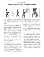
Fig. 1. A: a surface Ω ⊂ IR 3 and a set of points X ∈ IR 3 (picked on Ω in this 

example but it is not mandatory, they could be anywhere in IR 3 ). B: The 3d Voronoi 

diagram Vor(X) in IR 3 (cross-section). C: the 3d Voronoi diagram Vor(X) with the 

restricted Voronoi diagram Vor(X)∣ Ω superimposed. Each restricted Voronoi cell Ω i 

is the intersections between the 3d Voronoi cell Vor(x i) and the surface Ω (a closer 

view is shown in Figure 2). 

Restricted Voronoi Diagram 

We quickly introduce the notion of Restricted Voronoi Diagram, that plays 

a central role in several mesh generation algorithms (see e.g. [12] and the 

references herein). We consider a domain Ω ⊂ IR d . In our specific case, Ω 

will be a surface embedded in IR d (but the definitions below apply to any 

subset). The Voronoi diagram of X restricted to Ω, denoted by Vor(X)∣ Ω , is 

the collection of subsets Ω i of Ω defined by : 

Vor(X)∣ Ω = {Ω i } ; Ω i = Vor(x i ) ∩ Ω = {x ∈ Ω∣d(x, x i ) ≤ d(x, x j )∀j} . 

Fig. 2. A Restricted Voronoi Diagram with the associated Restricted Delaunay 

Triangulation superimposed.


A B C D 

Fig. 3. A: Voronoi diagram of a random pointset X (black dots), and centroids of the 

Voronoi cells (green dots). B: configuration after one iteration of Lloyd relaxation. 

C: after 100 iterations. D: Delaunay triangulation. 

The subset Ω i is called the restricted Voronoi cell of x i (see Figure 1). Similarly 

to the standard (unrestricted) case, one can define the dual of a restricted 

Voronoi diagram, called the Restricted Delaunay Triangulation (RDT 

for short). Each triangle of the RDT corresponds to three Restricted Voronoi 

Cells that have a non-empty intersection (see Figure 2). 

As a direct consequence of their definition, the restricted Voronoi cells can 

be also given by : 

Ω i = Ω ∩ (⋂ Π + (i, j)) 

j 

where Π + (i, j) = {x∣d(x, x i ) ≤ d(x, x j )} denotes the halfspace bounded by 

the bisector of the segment [x i , x j ] that contains x i . In other words, the 

Voronoi cell Ω i can be obtained by starting from the entire space Ω and 

iteratively clipping it with the bisectors Π + (i, j) defined by all other sites 

x j . Directly applying this iterative clipping procedure clearly has no practical 

value, since the resulting algorithm has superquadratic complexity. For this 

reason, most existing algorithms that compute Voronoi diagrams are based on 

different considerations, such as properties of the Delaunay triangulation (see 

[6] for a survey). However, computing a Delaunay triangulation has time and 

space complexity proportional to d!, where d denotes the dimension. While 

the d! constant is small for d = 2 or d = 3, in our context of anisotropic mesh 

generation, we use a higher dimensional space (d = 6 typically, see below), for 

which this d! time/space requirement is prohibitive. In Section 4, we will show 

a simple theorem that makes the iterative clipping point of view practical in 

our specific context, and that avoids the d! factor. 

Centroidal Voronoi Tessellation 

A Centroidal Voronoi Tessellation (CVT for short) is a Voronoi Diagram that 

satisfies the following property : 

∀i, x i = g i


where g i denotes the centroid of the Voronoi cell Ω i . A CVT can be computed 

by the so-called Lloyd relaxation [31], that iteratively moves each vertex x i to 

the centroid g i . Lloyd relaxation generates a regular sampling[18, 17], from 

which a Delaunay triangulation with well-shaped isotropic elements can be 

extracted [19, 21, 3]. An example of CVT and its dual Delaunay triangulation 

is shown in Figure 3. In the case of surface meshing, it is possible to 

generalize this definition by using a geodesic Voronoi diagram over the surface 

Ω [38], where the Euclidean distance d that appears in the definition 

of the Voronoi cells is replaced with the geodesic distance measured on the 

surface Ω. However, computing a geodesic Voronoi diagram is costly, and becomes 

prohibitive in our context, that require multiple iterations. The notion 

of Restricted Centroidal Voronoi Tessellation[20] can be used instead. The 

idea consists in letting the points x i move in the entire ambient space IR d , 

and replace the geodesic Voronoi diagram on Ω with the restricted Voronoi 

diagram VorX∣ Ω introduced above. The algorithm has the same structure as 

Lloyd relaxation in 3d (a 3d Voronoi diagram is computed). The only difference 

is that the centroids g i are computed from the restricted Voronoi cells 

Ω i = Vor(x i ) ∩ Ω instead of the full Voronoi cells Vor(x i ). Since the centroids 

are not necessarily on Ω, it may be required to reproject them onto 

Ω after each iteration (hence defining a Constrained CVT). With an efficient 

algorithm to compute the Restricted Voronoi Diagram, Restricted and Constrained 

CVT can be used for isotropic surface remeshing [44]. We will show 

further how Restricted CVT can be implemented in higher-dimensional space 

and used to optimize all the vertices of an anisotropic mesh simultaneously. 

2.2 Anisotropy 

Definition 

We consider now that a metric G(.) is defined over the domain IR d . In other 

words, at a given point x ∈ IR d , the dot product between two vectors v and 

w is given by : 

< v, w > G(x) = v t G(x)w. 

In practice, the metric G(x) can be represented by a symmetric d × d matrix 

(with coefficients that possibly vary in function of the coordinates of x). 

Given a metric G and an open curve C ⊂ IR d , it is possible to define the 

length of C relative to G as : 

l G (C) = ∫ 

1 

t=0 

√ 

v(t)t G(x(t))v(t)dt 

where x(.) denotes a parameterization of C and v(t) = ∂x(t)/∂t the tangent 

vector. Then, the anisotropic distance d G (x, y) between two points x and y


is defined as the length of the (possibly non-unique) shortest curve C that 

connects x and y : 

d G (x, y) = min l G(C). 

{C∣C(0)=x,C(1)=y} 

Since d G (., .) is very difficult to compute in practice, some methods also 

use the (simpler to compute) anisotropic length of the segment (x, y) : 

¯d G (x, y) = l G ([x, y]) 

Relation with the Theory of Approximation and Applications 

Anisotropy is related with the theory of approximation[15, 39], that studies 

how to best approximate a function with a given budget of points. Under 

some circumstances, it is possible to characterize the anisotropy of the optimal 

mesh, and design algorithms to optimize the approximation properties 

of a mesh. Some methods based on an anisotropic version of point insertion 

in Delaunay triangulation were proposed and successfully applied to many 

practical cases [8, 9, 7, 16]. The continuous mesh framework [32, 33] is based 

on an equivalence between some set of ellipses circumscribed to the triangles 

of a mesh and a continuous metric. In this setting, a metric is considered 

as the “limit case” of a mesh with infinitely small anisotropic triangles. In 

practice, this consideration results in highly efficient anisotropic mesh adaptation 

algorithms. The connections between anisotropic meshes and approximation 

theory were studied, not only for piecewise linear functions, but also 

for higher-order finite elements [34, 35, 13]. This theoretical analysis leads to 

an efficient greedy bissection algorithm that generates optimal meshes. In the 

specific case of computing a polygonal approximation of a given shape, some 

metrics were proposed[14, 42], together with discrete (per-facet) Lloyd-like 

optimization algorithms. 

Anisotropic Generalizations of Voronoi Diagrams 

Our goal is to experiment Lloyd relaxation in the anisotropic setting, with 

a continuous formulation, independent on the shape of the original triangles. 

Thus, we need a definition of Voronoi diagrams that accounts for anisotropy. 

The most general setting is given by Riemann Voronoi diagrams [28], that 

replace the distance d(x, y) with the anisotropic distance d G (x, y) defined 

above. Some theoretical results are known, however, a practical implementation 

in 3d is still beyond reach. For this reason, two simplifications are used : 

Vor Labelle (x i ) = {y∣d xi (x i , y) ≤ d xj (x j , y)∀j} 

Vor Du (x i ) 

= {y∣d y (x i , y) ≤ d y (x j , y)∀j} 

where: d x (y, z) = √ (z − y) t G(x)(z − y)


A B C 

Fig. 4. Anisotropic Voronoi Diagram and Delaunay Triangulation. A: prescribed 

anisotropy field; B: anisotropic Voronoi diagram and C: Delaunay triangulation. 

The first definition Vor Labelle [27] defines an object that is easier to analyze 

theoretically. The bisectors are quadratic surfaces, known in closed form, 

and a provably correct Delaunay refinement algorithm can be defined. The 

so-defined anisotropic Voronoi diagram may be also thought of as the projection 

of a higher-dimensional power diagram [5]. The second definition Vor Du 

[22] is best suited to a practical implementation of Lloyd relaxation. In particular, 

the midpoints can be determined. An approximation of the Voronoi 

cells and their centroids can be reasonably easily computed for 2d domains 

and parametric surfaces. However, generalizing the algorithms to arbitrary 3d 

surfaces may be difficult. 

In what follows, we propose a general method to apply Lloyd relaxation 

to a surface embedded in a higher dimensional space. For a given arbitrary 

metric G (e.g. for solution-based adaptivity), one may use the embedding 

defined in [5]. In this paper, though the algorithm may be applicable to more 

general settings, we will limit ourselves to a simpler embedding explained in 

the next section, well suited to generate curvature-adapted surfacic meshes. 

3 Trading Anisotropy for Additional Dimensions 

3.1 A simple example 

We consider the 2d metric G depicted in Figure 4-A. The deformed circles correspond 

to the points equidistant to the black dots in terms of the distance d G 

defined by the metric. Our goal is to generate an anisotropic Voronoi diagram 

governed by this metric (Figure 4-B) and deduce an anisotropic mesh from its 

dual (Figure 4-C). For this simple example, one can see that Figures 4-A,B,C 

can be considered as the surfaces in Figures 5-A,B,C (next page) “seen from 

above”. In other words, by embedding the flat 2d domain as a curved surface 

in 3d, one can recast the anisotropic meshing problem as the isotropic meshing


A B C 

Fig. 5. A 3d surface that generates the prescribed anisotropy in Figure 4 when 

“seen from above” (in general, more dimensions are needed). 

of a surface embedded in higher-dimensional space. Isotropic surface meshing 

can be computed as a restricted CVT (see the previous section). 

In general (i.e., for an arbitrary metric G), a higher-dimensional space 

will be needed [37]. In the case of 3d surface or volume meshing, using Labelle 

and Shewchuk’s discrete definition of anisotropic Voronoi diagrams with 

Boissonnat et.al’s characterization[5], one needs dimension d = 10 (it uses a 

power diagram of dimension 9 that can be seen as the projection of a Voronoi 

diagram of dimension 10). For this reason, we propose an algorithm to compute 

a restricted CVT of a surface embedded in higher-dimensional space. 

Before presenting the algorithm, we present a simple embedding, well suited 

to generate curvature-adapted anisotropic mesh. 

3.2 The Gauss map 

In this section, we present a 6d embedding, that uses both positions and 

normals. This embedding was used to generate anisotropic quad meshes by 

contouring in 6d[10], to classify the features of meshes[26] or to compute 

anisotropic quadrangulations[25]. It has interesting connections with surface 

normal approximation[11]. 

Given a surface Ω ⊂ IR 3 , the Gauss map is the application that maps Ω 

onto the unit sphere S 2 , defined by x ∈ Ω ↦ n(x) ∈ S 2 , where n(x) denotes 

the unit normal vector at x. The Gauss map plays a fundamental role in 

the definition of curvature. For instance, Gauss curvature is defined as the 

Jacobian of the Gauss map. In other words, Gauss curvature is a measure 

of how areas are locally distorted by the Gauss map. As a consequence, a 

uniform sampling of the unit sphere results in a curvature-adapted mesh when 

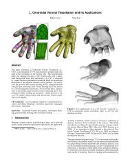
transformed back onto Ω. As shown in Figure 6, the tips of the fingers cover 

a wide area of the unit sphere when transformed by the Gauss map, and 

therefore have a high density of vertices in the sampling (region a in the 

figure). In contrast, the tubular regions of the fingers (region b) just cover an


Fig. 6. A: a surface with two highlighted zones (a and b). B: the Gauss map of zones 

a and b (dark gray). Zone a covers half of the sphere, whereas zone b only covers an 

annulus around the equator of the sphere. C: an isotropic meshing in Gauss space 

mapped back into Euclidean space is a curvature-adapted anisotropic mesh. Zone a 

contains more vertices than zone b since it covers a larger space in the Gauss map. 

annulus around the equator of the unit sphere. A uniform sampling of this 

annulus, when transformed back onto Ω, results in triangles that are elongated 

along the axis of the tubular region. Unfortunately, for general surfaces (i.e. 

non-convex), the Gauss map is not bijective. For this reason, we propose 

instead to use the embedding Φ ∶ Ω → IR 6 defined by: 

⎡ 

x ⎤ ⎥⎥⎥⎥⎥⎥⎥⎥⎥⎥⎦ 

y 

Φ(x) = 

z 

sn x 

sn y 

⎢ 

⎣ sn z 

where n x , n y , n z denotes the normal to Ω at x, and where s ∈ (0, +∞) is a 

constant, user-defined factor that specifies the desired amount of anisotropy. 

For a small value of s, the normal components are ignored, and an isotropic 

mesh is obtained. For high values of s, more importance is given to the Gauss 

map components, and a highly anisotropic mesh is obtained. In what follows, 

we will use this embedding. Other embeddings can account for different 

anisotropies. They will be discussed in conclusion. 

We now consider a surface Ω given as a triangle mesh. One can evaluate 

the normals at the vertices of Ω, and embed Ω into IR 6 with Φ. At this point, 

a possibility would be to use Algorithm 1 below. Step 1 is detailed further in 

Section 4.2. Step 2 may use an implementation of Delaunay triangulation in 

arbitrary dimension, available in QHull[4] or as an experimental package of 

CGAL[1]. Step 3 could use two nested loops, one over the m facets of Ω and


(1) X ← initial random sampling of Ω in IR 6 

while minimum not reached do 

(2) Compute the Voronoi diagram V or(X) in IR 6 

(3) Compute the restricted Voronoi diagram V or(X)∣ Ω 

foreach i do 

Compute g i = ∫ Ωi 

xdx/ ∫ Ωi 

dx 

x i ← g i 

end 

end 

Algorithm 1: Naive implementation of anisotropic CVT in IR 6 

one over the n Voronoi cells of Vor(X). The O(mn) complexity of these two 

nested loops can be replaced with O(m + n), by a propagation along both the 

facet graph of Ω and the cell graph of Vor(X)[44]. This propagation generates 

all couples (f, i) such that the Voronoi cell Vor(x i ) has a non-empty intersection 

with the facet f. From the (f, i) couples, the restricted Voronoi cells Ω i 

are obtained by accumulating the contributions of all facets Vor(x i ) ∩ f. 

Our experiments with this approach, for d = 6 and n = 5000 vertices showed 

that 100 iterations of Lloyd relaxation requires more than a day, even with 

a high-end 16Gb computer, that exhausts its physical memory and starts 

swapping (due to the d! cost in memory). For this reason, we propose an 

alternative in the next section, that not only avoids the d! cost, but also 

can be easily parallelized. Our algorithm scales-up well and can optimize an 

anisotropic mesh with one million vertices in minutes on an 8 cores machine. 

4 CVT in high-dimensional space with Vorpaline 

The basic operation in the step 3 of Algorithm 1 above consists in clipping a 

facet of Ω with a Voronoi cell of Vor(X). A Voronoi cell is a convex polytope, 

that can be defined as the intersection of halfspaces : 

Vor(x i ) = 

v i 

⋂ 

k=1 

Π + (i, j k ) 

where Π + (i, j) denotes the halfspace bounded by the bisector of (x i , x j ) that 

contains x i , the j k ’s denote the indices of the v i Voronoi cells that have a 

facet (of dimension d − 1) in common with Vor(x i ). In terms of Delaunay 

triangulation, they correspond to the indices of the vertices connected to x i 

by a Delaunay edge (and v i denotes the valence of the vertex i in the Delaunay 

1-skeleton). This representation of the Voronoi cells (H-representation) is well 

suited to the computation of the intersections with the facets of Ω in step 

3, that can be efficiently computed by Sutherland & Hodgman’s re-entrant 

clipping[40].


Vor(xi) 

xi 

xj 

Fig. 7. The Voronoi cell Vor(x i) is the result of clipping the entire space by all 

the bisectors (continuous lines) of the segments [x i, x j] (dashed lines). Among the 

bisectors, some are contributing (black) and some are non-contributing (gray). 

Alternatively, as indicated in Section 2.1, the definition of the Voronoi cell 

Vor(x i ) directly gives : 

Vor(x i ) = ⋂ Π + (i, j) 

j≠i 

One can see that all the possible bisectors are used, in contrast with the 

previous definition of Vor(x i ) that only uses the neighbors. As a consequence, 

we can classify the bisectors Π + (i, j) into two sets (see Figure 7). 

The bisector Π + (i, j) is said to be : 

ˆ non-contributing if Vor(x i ) ⊂ Π + (i, j) ; 

ˆ contributing otherwise. 

In other words, clipping a Voronoi cell by a non-contributing bisector does not 

change the result. Therefore, the Voronoi cell can be computed by intersecting 

a superset of the contributing bisectors. We now propose an algorithm that 

provably finds all the contributing bisectors of a Voronoi cell. 

4.1 Radius of Security 

We now suppose that the vertices X are organized in a geometric search data 

structure, such that for any x i one can efficiently compute the list of nearest 

neighbors x j sorted by increasing distance to x i . We use the ANN 3 library 

[36]. The algorithm in ANN has linear space-time complexity for construction 

in function of both the number of points and the dimension, and O(d log(n)) 

complexity for nearest neighbors queries. 

3 Approximate Nearest Neighbors. Note: it returns exactly the nearest neighbors 

when the parameter ɛ is set to 0.


Let x j1 , x j2 , . . . x jn−1 denote the vertices sorted by increasing distance from 

x i . Let V k denote the intersection of the k first bisectors and R k denote its 

x i -centered radius : 

V k (x i ) = ⋂ 

k Π + (i, j l ) 

l=1 

R k = max{d(x i , x)∣x ∈ V k (x i )}. 

We have then the following simple theorem : 

Theorem 1. For all j such that d(x i , x j ) > 2R k , the bisector Π + (i, j) is noncontributing, 

i.e. V k (x i ) ⊂ Π + (i, j). 

Proof. Consider x ∈ V k (x i ) and x j such that d(x i , x j ) > 2R k . 

By definition of R k , d(x, x i ) < R k . 

We have d(x i , x) + d(x, x j ) > (x i , x j ) (triangular inequality) 

and d(x i , x j ) > 2R k , 

therefore d(x, x j ) > R k > d(x, x i ) and x ∈ Π + (i, j) 

∎ 

As a direct consequence of Theorem 1 : 

d(x i , x jk+1 ) > 2R k ⇒ V k = Vor(x i ). 

We call radius of security the first value of R k that satisfies this condition. 

Note that this theorem does not have a practical value in the case of the 

(unrestricted) Voronoi diagram, since some cells are unbounded and have 

infinite R k (therefore, for an infinite cell, all the bisectors are considered), 

leading to prohibitive computation time. However, it is clear that the theorem 

applies to the restricted Voronoi diagram Vor(X)∣ Ω . It also gives a practical 

way of computing Vor(x i ) ∩ f for a bounded set f (e.g., a facet of Ω). This 

configuration is detailed in Algorithm 2, that we will use to compute restricted 

CVT in IR d . 

Data: a facet f = (p 1, p 2, p 3) of Ω and a set of points X ∈ IR d 

Result: V = Vor(x i) ∩ f 

V ← f 

R ← max{d(x i, p 1), d(x i, p 2), d(x i, p 3)} 

k ← 1 

while d(x i, x jk ) < 2R and k < n do 

V ← V ∩ Π + (i, j k ) 

R ← max{d(x, x i)∣x ∈ V } 

k ← k + 1 

end 

Algorithm 2: Clipping a facet with a Voronoi cell in IR d .


Data: a surface Ω, the desired number of points n and anisotropy s 

Result: an anisotropic sampling X of Ω 

(1) embed Ω in IR 6 using Φ s (see Section 3.2) 

(2) compute an initial random sampling X in IR 6 (see Algorithm 4 below) 

for k = 1 to nbiter do 

Update the ANN data structure with X 

g 1...n ← 0 ; m 1...n ← 0 

(3) foreach {(t, x i)∣t ∩ Vor(x i) ≠ ∅} do 

(4) V ← t ∩ Vor(x i) (Algorithm 2) 

(5) m ← mass(V ) ; m i ← m i + m ; g i ← g i + m × centroid(V ) 

end 

for i = 1 to n do 

(6) x i ← 1/m i × g i 

end 

end 

Algorithm 3: Anisotropic Lloyd Relaxation in IR d 

4.2 Implementation 

Anisotropic Lloyd relaxation is detailed in Algorithm 3. Step (3) is based on 

a recursive propagation on the facet graph of Ω and the cell graph of Vor(X) 

detailed in [44]. The mass (measure in 6d) and centroid of each clipped facet 

is accumulated in intermediary variables, from which the centroids are computed 

(5),(6). Finally, the Restricted Delaunay triangulation is computed as 

the dual of the Restricted Voronoi Diagram, (or the dual of its connected 

components[29] to avoid some degenerate configurations). Note that convergence 

can be significantly accelerated by replacing Lloyd relaxation with quasi- 

Newton optimization[30]. The latter was used in the results shown in this 

paper. 

Initialization is computed as in Algorithm 4. In step (1), the area of a triangle 

in IR d can be computed with Heron’s formula A = √ s(s − a)(s − b)(s − c) 

Data: a surface Ω embedded in IR d and the desired number of points n 

Result: an initial sampling X of Ω 

Generate a vector (s i) of n random numbers 

Sort (s i) 

(1) foreach f ∈ Ω, compute the normalized area a f = Area(f)/ ∑ f Area(f) 

f ← 1 ; A ← 0 

for i = 1 to n do 

while (s i > A) f ← f + 1 ; A ← A + a f 

(2) x i ← random point in f 

end 

Algorithm 4: Computing the initial random sampling in IR d


where a, b, c denote the length of the three edges and s = a + b + c. Step (2) 

uses Turk’s method to generate a random point in a triangle[41]. 

Due to space constraints, the implementation is not fully detailed here 

(but will be in a future publication). We outline two important aspects : 

ˆ 

ˆ 

parallelism : the computation of a specific Voronoi cell is independent on 

the others. Thus, we first partition the input surface into N parts (typically 

N = number of cores) with METIS[23]. We use one thread per part to 

compute the masses and centroids of the restricted Voronoi cells in each 

part (Alg. 3 (3)-(5)). Finally, each point x i is updated by accumulating 

the contribution of each part to the centroid of its restricted Voronoi cell. 

genericity : Our implementation is based on C++ templates, in the spirit 

of CGAL[1] library. With a “Kernel” class, we parameterize the algorithm 

in terms of dimension d (that can be known at compile time or dynamic) 

and exact geometric predicates (that use arithmetic filters). 

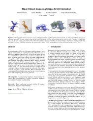
5 Results 

We have experimented our implementation on several databases, comprising 

CAD data and scanned meshes. Some representative results are shown in 

Figure 8 and 9. To compute the embedding, we used the normal to the CAD 

surface whenever available, or estimated it at the vertices of the input triangle 

mesh for scanned meshes. Input meshes have between 30K and 4M triangles. 

We have generated anisotropic meshes with up to 1M vertices. Computation 

time ranges between a few seconds and 10 minutes for 100 iterations of Newton 

optimization on a 8-cores PC. 

6 Discussion, Conclusions and Future Work 

We proposed an efficient methodology to implement Lloyd relaxation in high 

dimensional space, and applications to anisotropic surface remeshing. A limitation 

of our method is that the Restricted Delaunay Triangulation may 

contain flipped triangles, in particular in zones where the direction of the 

anisotropy varies too quickly. This difficulty is pointed-out in [27]. This may 

be fixed with some post-processing (e.g. Delaunay refinement). Another limitation 

concerns creases and sharp features, that are oversampled in the direction 

orthogonal to the crease. We think that this issue can be solved by 

explicitely sampling the creases, then using constrained optimization combined 

with “protecting balls” [12]. This means computing a power diagram, 

that can be obtained from a d + 1 Voronoi diagram in which our “security radius” 

theorem can be used. We also mention that our algorithmic framework 

can be easily adapted to tetrahedral meshes embedded in nd, by replacing the 

3d tetrahedral clipping routine in [43] by our nd Vorpaline method. This may 

be used to generate 3d anisotropic tetrahedral meshes.


Fig. 8. Anisotropic meshes - mechanical parts. 

In a more general perspective, this work shows the practicality of geometric 

computing in high-dimensional space, and in particular the possibility of 

computing a restricted Voronoi diagram in IR d . Besides the 6d (Euclidean × 

Gauss-map) embedding experimented here, we plan to experiment with more 

general metric fields and the 10d embedding [5]. 

We also conducted experiments with a much larger number of coordinates, 

obtained by the Finite Element discretization of the eigenfunctions of a symmetric 

operator. This allows to implement CVT for kernel-based distances. In 

our preliminary results, with our generic implementation, we obtained reasonable 

timings (minutes) for remeshing in dimension spaces as large as d = 5000.


Fig. 9. Anisotropic meshes - scanned data. 

Acknowledgments 

This work is partly supported by the European Research Council (GOOD- 

SHAPE, ERC-StG-205693), the ANR (MORPHO) and NSF (grant IIS 11109555). 

The authors wish to thank Wenping Wang for many discussions. The meshes 

shown in the paper are courtesy of Jean-François Remacle, Christophe Geuzaine, 

Nicolas Saugnier and AimAtShape. The F1 car is from www.opencascade.org. 

References 

1. CGAL. http://www.cgal.org. 

2. Frédéric Alauzet and Adrien Loseille. High-order sonic boom modeling based 

on adaptive methods. J. Comput. Physics, 229(3):561–593, 2010. 

3. P. Alliez, E. Colin de Verdière, O. Devillers, and M. Isenburg. Centroidal 

Voronoi diagrams for isotropic remeshing. Graphical Models, 67(3):204–231, 

2003. 

4. C. Bradford Barber, David P. Dobkin, and Hannu Huhdanpaa. The quickhull 

algorithm for convex hulls. ACM Transactions on Mathematical Software, 

22(4):469–483, 1996.


5. J.-D. Boissonnat, C. Wormser, and M. Yvinec. Anisotropic Diagrams: Labelle 

Shewchuk approach revisited. Theo. Comp. Science, (408):163–173, 2008. 

6. Jean-Daniel Boissonnat and Mariette Yvinec. Algorithmic Geometry. Cambridge 

University Press, 1998. 

7. H. Borouchaki and P.-L. George. Delaunay Triangulation and Meshing: Application 

to Finite Elements. Hermès, 1998. 

8. H. Borouchaki, P.-L. George, F. Hecht, P. Laug, and E. Saltel. Delaunay mesh 

generation governed by metric specifications. part 1: Algorithms. Finite Elements 

in Analysis and Design, 25:61–83, 1997. 

9. H. Borouchaki, P.-L. George, F. Hecht, P. Laug, and E. Saltel. Delaunay mesh 

generation governed by metric specifications. part 2: Application examples. Finite 

Elements in Analysis and Design, 25:85–109, 1997. 

10. Guillermo D. Canas and Steven J. Gortler. Surface remeshing in arbitrary 

codimensions. Vis. Comput., 22(9):885–895, September 2006. 

11. Guillermo D. Canas and Steven J. Gortler. Shape operator metric for surface 

normal approximation. In International Meshing Roundtable Conference Proceedings, 

Salt Lake City, November 2009. 

12. Siu-Wing Cheng, Tamal K. Dey, and Joshua A. Levine. A practical delaunay 

meshing algorithm for alarge class of domains. In 16th International Meshing 

Roundtable conf. proc., pages 477–494, 2007. 

13. A. Cohen, N. Dyn, F. Hecht, and J.-M. Mirebeau. Adaptive multiresolution 

analysis based on anisotropic triangulations. Math. Comput., 81(278), 2012. 

14. David Cohen-Steiner, Pierre Alliez, and Mathieu Desbrun. Variational shape 

approximation. ACM Transactions on Graphics, 23:905–914, 2004. 

15. E. d’Azevedo. Optimal triangular mesh generation by coordinate transformation. 

Technical report, University of Waterloo, 1989. 

16. Cécile Dobrzynski and Pascal J. Frey. Anisotropic Delaunay mesh adaptation 

for unsteady simulations. In Proceedings of the 17th international Meshing 

Roundtable, pages 177–194, États-Unis, 2008. 

17. Qiang Du, Maria Emelianenko, and Lili Ju. Convergence of the Lloyd algorithm 

for computing centroidal Voronoi tessellations. SIAM Journal on Numerical 

Analysis, 44(1):102–119, 2006. 

18. Qiang Du, Vance Faber, and Max Gunzburger. Centroidal Voronoi tessellations: 

applications and algorithms. SIAM Review, 41(4):637–676, 1999. 

19. Qiang Du and Max Gunzburger. Grid generation and optimization based on 

centroidal Voronoi tessellations. Applied Mathematics and Computation, 133(2- 

3):591–607, 2002. 

20. Qiang Du, Max. D. Gunzburger, and Lili Ju. Constrained centroidal Voronoi 

tesselations for surfaces. SIAM Journal on Scientific Computing, 24(5):1488– 

1506, 2003. 

21. Qiang Du and Desheng Wang. Tetrahedral mesh generation and optimization 

based on centroidal Voronoi tessellations. International Journal for Numerical 

Methods in Engineering, 56:1355–1373, 2003. 

22. Qiang Du and Desheng Wang. Anisotropic centroidal Voronoi tessellations and 

their applications. SIAM Journal on Scientific Computing, 26(3):737–761, 2005. 

23. George Karypis and Vipin Kumar. Metis - unstructured graph partitioning and 

sparse matrix ordering system, version 2.0. Technical report, 1995. 

24. William Kleb. Nasa technical brief - advanced computational fluid dynamics 

and mesh generation, 2009. http://www.techbriefs.com/component/content/ 

article/5075.


25. Denis Kovacs, Ashish Myles, and Denis Zorin. Anisotropic quadrangulation. In 

Proceedings of the 14th ACM Symposium on Solid and Physical Modeling, SPM 

’10, pages 137–146, New York, NY, USA, 2010. ACM. 

26. Yu kun Lai, Qian yi Zhou, Shi min Hu, Johannes Wallner, and Helmut 

Pottmann. Robust feature classification and editing. IEEE Trans. Visualization 

and Computer Graphics, 2007. 

27. F. Labelle and J.-R. Shewchuk. Anisotropic Voronoi diagrams and guaranteedquality 

anisotropic mesh generation. In SCG ’03: Proceedings of the nineteenth 

annual symposium on Computational geometry, pages 191–200, 2003. 

28. Greg Leibon and David Letscher. Delaunay triangulations and voronoi diagrams 

for riemannian manifolds. In SCG conf. proc., pages 341–349. ACM. 

29. Bruno Lévy and Yang Liu. Lp Centroidal Voronoi Tesselation and its applications. 

ACM Transactions on Graphics, 29(4), 2010. 

30. Yang Liu, Wenping Wang, Bruno Lévy, Feng Sun, Dong-Ming Yan, Lin Lu, and 

Chenglei Yang. On centroidal Voronoi tessellation—energy smoothness and fast 

computation. ACM Transactions on Graphics, 28(4):1–17, 2009. 

31. Stuart P. Lloyd. Least squares quantization in PCM. IEEE Transactions on 

Information Theory, 28(2):129–137, 1982. 

32. Adrien Loseille and Frédéric Alauzet. Continuous mesh framework part i: Wellposed 

interpolation error. SIAM J. Numerical Analysis, 49(1):38–60, 2011. 

33. Adrien Loseille and Frédéric Alauzet. Continuous mesh framework part ii: Validations 

and applications. SIAM J. Numerical Analysis, 49(1):61–86, 2011. 

34. Jean-Marie Mirebeau and Albert Cohen. Anisotropic smoothness classes: From 

finite element approximation to image models. Journal of Mathematical Imaging 

and Vision, 38(1):52–69, 2010. 

35. Jean-Marie Mirebeau and Albert Cohen. Greedy bisection generates optimally 

adapted triangulations. Math. Comput., 81(278), 2012. 

36. D. M. Mount and S. Arya. ANN: A library for approximate nearest neighbor 

searching. In CGC Workshop on Computational Geometry, pages 33–40, 1997. 

37. J. F. Nash. The imbedding problem for riemannian manifolds. Annals of Mathematics, 

63:20–63, 1956. 

38. Gabriel Peyré and Laurent Cohen. Surface segmentation using geodesic centroidal 

tesselation. In 2nd International Symposium on 3D Data Processing, 

Visualization and Transmission (3DPVT 2004), pages 995–1002, 2004. 

39. Jonathan Richard Shewchuk. What is a good linear finite element? - interpolation, 

conditioning, anisotropy, and quality measures. Technical report, In Proc. 

of the 11th International Meshing Roundtable, 2002. 

40. Ivan Sutherland and Gary W. Hodgman. Reentrant polygon clipping. Communications 

of the ACM, 17:32–42, 1974. 

41. Greg Turk. Graphics gems. chapter Generating random points in triangles, 

pages 24–28. Academic Press Professional, Inc., San Diego, CA, USA, 1990. 

42. Sébastien Valette, Jean-Marc Chassery, and Rémy Prost. Generic remeshing of 

3D triangular meshes with metric-dependent discrete Voronoi diagrams. IEEE 

Transactions on Visualization and Computer Graphics, 14(2):369–381, 2008. 

43. D.-M. Yan, W. Wang, B. Lévy, and Y. Liu. Efficient computation of 3d clipped 

voronoi diagram. In GMP conf. proc., pages 269–282, 2010. 

44. Dong-Ming Yan, Bruno Lévy, Yang Liu, Feng Sun, and Wenping Wang. Isotropic 

remeshing with fast and exact computation of restricted Voronoi diagram. Computer 

Graphics Forum, 28(5):1445–1454, 2009.

Variational Anisotropic Surface Meshing with Voronoi Parallel ...

You also want an ePaper? Increase the reach of your titles

Delete template?

Save as template?