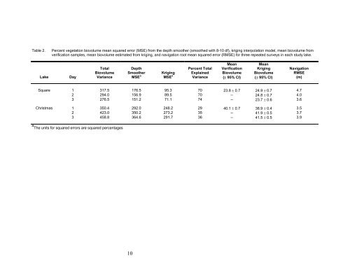
Table 2. Percent vegetation biovolume mean squared error (MSE) from the depth smoother (smoothed with 8-10 df), kriging interpolation model, mean biovolume from verification samples, mean biovolume estimated from kriging, <strong>and</strong> navigation root mean squared error (RMSE) for three repeated surveys in each study lake. Lake Day Total Biovolume Variance Depth Smoother MSE a Kriging MSE a Percent Total Explained Variance Mean Verification Biovolume (± 95% CI) Mean Kriging Biovolume (± 95% CI) Navigation RMSE (m) Square 1 317.5 176.5 95.3 70 23.8 ± 0.7 24.9 ± 0.7 4.7 2 294.0 156.9 89.5 70 -- 24.8 ± 0.7 4.0 3 276.5 151.2 71.1 74 -- 23.7 ± 0.6 3.6 Christmas 1 350.4 292.0 248.2 29 40.1 ± 0.7 38.9 ± 0.4 3.5 2 423.0 350.2 273.2 35 -- 41.9 ± 0.5 3.7 3 458.8 364.6 291.7 36 -- 41.5 ± 0.5 3.9 a The units for squared errors are squared percentages 10
much smaller than our reported errors. However, it is important to note that error estimations from Sabol et al. (2002) represent differences between average predicted <strong>and</strong> average observed plant heights within ensonified 0.3m x 0.3m quadrats, <strong>and</strong> not over individual plants like our fixed-point experiments. Because Sabol et al. (2002) averaged data over larger sampling units than our study, the central limit theorem, in part, may explain their smaller errors. Whole-lake surveys–Our methods produced consistently accurate <strong>and</strong> precise maps <strong>of</strong> biovolume for Square Lake. For Christmas Lake, maps were accurate but not precise. These results for Christmas Lake are contrary to results published by Valley et al. (2005) that documented high map precision in this lake. However, in our earlier study, we extended analyses to a depth <strong>of</strong> 8 m in both Square <strong>and</strong> Christmas lakes. This depth was an appropriate cut-<strong>of</strong>f for analyses in Square Lake because vegetation usually covered all bottom areas close to 8 m deep. However, in Christmas Lake, vegetation was sparse beyond 6.2 m. Biovolume in areas between 6.2 m <strong>and</strong> 8 m in Christmas lake was <strong>of</strong>ten zero, thus artificially inflating map precision. The effect <strong>of</strong> analysis boundaries on statistical distributions illustrates the importance <strong>of</strong> carefully defining the boundaries <strong>of</strong> the littoral zone. Morris (1992) defined the littoral zone as the area <strong>of</strong> shallow fresh water in which light penetrates to the bottom <strong>and</strong> nurtures rooted plants. Our operational definition as a zone <strong>of</strong> contiguous bottom cover by vegetation fits this concept. Valley et al. (2005) demonstrated that the degree <strong>of</strong> agreement between verification <strong>and</strong> predicted data increased as littoral depth increased. Similarly, in this analysis, as depth increased, our survey precision increased as well. Lower survey <strong>and</strong> map precision at shallow depths is not surprising given the suite <strong>of</strong> localized disturbances that cause vegetation patchiness in such areas (e.g., harvesting, sedimentation, wind/ice scour). In addition, small deviations in plant height in shallow depths lead to large deviations in biovolume. As a result, we suggest focusing greater sampling effort at depths less than two meters <strong>and</strong> less effort at deeper depths. Fortunately, kriging is not greatly affected by unbalanced survey designs, <strong>and</strong> its behavior as a smoother makes it robust to modest environmental noise (Isaaks <strong>and</strong> Srivastava 1989). Ultimately, the scale <strong>of</strong> the question <strong>and</strong> level <strong>of</strong> spatial resolution supported by the data must be carefully considered prior to interpreting results. REFERENCES Burks, R. L., E. Jeppesen, <strong>and</strong> D. M. Lodge. 2001. Littoral zone structures as Daphnia refugia against predators. Limnolology <strong>and</strong> Oceongraphy 46:230-237. Christensen, D. L., B. R. Herwig, D. E. Shindler, S. R. Carpenter. 1996. Impacts <strong>of</strong> lakeshore residential development on coarse woody debris in north temperate lakes. Ecological Applications 6:1143-1149. Canfield, D. E., J. V. Shireman, D. E. Colle, W. T. Haller, C. E. Watkins II, <strong>and</strong> M. J. Maceina. 1984. Prediction <strong>of</strong> chlorophyll a concentrations in Florida lakes: importance <strong>of</strong> aquatic macrophytes. Canadian Journal <strong>of</strong> Fisheries <strong>and</strong> Aquatic Sciences 41:497-501. Collins, W. T., R. S. Gregory, <strong>and</strong> J. T. Anderson. 1996. A digital approach to seabed classification. Sea Technology 37: 83-87. Drake, M. T., <strong>and</strong> R. D. Valley. 2005. Validation <strong>and</strong> application <strong>of</strong> a fish-based index <strong>of</strong> biotic integrity for small central Minnesota lakes. North American Journal <strong>of</strong> Fisheries Management 25:1095-1111. Duarte, C. M. 1987. 1987. Use <strong>of</strong> echosounder tracings to estimate the aboveground biomass <strong>of</strong> submerged plants in lakes. Canadian Journal <strong>of</strong> Fisheries <strong>and</strong> Aquatic Sciences 44:732-735. Isaaks, E. H., <strong>and</strong> R. M. Srivastava. 1989. An introduction to applied geostatistics, Oxford University Press, New York. Jennings, M. J., M. A. Bozek, G. R. Hatzenbeler, E. E. Emmons, M. D. Staggs. 1999. Cumulative effects <strong>of</strong> incremental shoreline habitat modification 11