Accuracy and Precision of Hydroacoustic Estimates ... - BioSonics, Inc

Minnesota Department of Natural Resources
Investigational Report 527, December 2005
ACCURACY AND PRECISION OF HYDROACOUSTIC ESTIMATES OF
AQUATIC VEGETATION AND THE REPEATABILITY OF WHOLE-LAKE
SURVEYS: FIELD TESTS WITH A COMMERCIAL ECHOSOUNDER 1
Ray D. Valley* and Melissa T. Drake
Minnesota Department of Natural Resources
Division of Fisheries and Wildlife
1200 Warner Road
St. Paul, MN 55106
Abstract- Hydroacoustics, coupled with GPS and GIS represents a promising tool in
monitoring changes to submersed vegetation biovolume, which is important for many Minnesota
fish species. However, prior to establishing operational survey programs using these
technologies, the performance of the equipment, software, and survey methodology must be
rigorously evaluated. Accordingly, we conducted ground-truth experiments with a BioSonics
Inc. digital echosounder by comparing estimates of bottom depth, plant height, and depth to
the top of the plant made with EcoSAV ® vegetation analysis software with measurements
made with divers. EcoSAV-estimated and diver-measured plant heights did not differ significantly,
however, the EcoSAV-estimated position of the plant in the water column did differ
from the diver-measured position. On average, EcoSAV over-estimated bottom depth by 0.18
m and over-estimated the depth from the surface to the top of the plant by 0.23 m. As a result,
the EcoSAV estimates indicated that plants occupied less of the water column than divermeasured
values. Bias in bottom measurements was likely due to signal penetration of the
soft sediments in Square Lake by the echosounder. Bias in top of plant measurements was
likely a result of difficulty placing the transducer directly over the marker buoys, so the top of
the plant sometimes fell outside and above the acoustic cone. We also evaluated whether
boat navigation error affected the accuracy and precision of vegetation maps, and the repeatability
of whole-lake surveys. To do so, we conducted surveys on three consecutive days in
two diversely vegetated lakes. Boat navigation RMSE averaged 3.5 to 4.0 meters; however,
GPS location error was only ± 1.06 m. These errors had little effect on the overall accuracy
and precision of maps of biovolume in both lakes. Precision of biovolume estimates was
lower at depths less than 2 meters than at deeper depths.
*Corresponding author: phone 651-793-6539, fax 651-772-7974, e-mail ray.valley@dnr.state.mn.us
1 This project was funded in part by the Federal Aid in Sport Fish Restoration (Dingell-Johnson) Program. Completion Report, Study 639,
D-J Project F-26-R Minnesota.
1

INTRODUCTION
Submersed aquatic vegetation provides
critical habitat for numerous Minnesota fish
species and is an integral component of fish
community integrity (Valley et al. 2004;
Drake and Valley 2005). The cumulative effects
of lakeshore and watershed development
has had negative effects on fish communities
in the upper Midwest (Christensen et al. 1996;
Jennings et al. 1999; Radomski and Goeman
2001; Drake and Valley 2005). Unfortunately,
habitat assessment techniques have lagged
behind impacts occurring to lake habitats,
and spatially explicit quantitative data on the
distribution of aquatic vegetation in lakes is
lacking. Hydroacoustics coupled with differentially
corrected GPS, analyzed in a GIS
represents a promising new tool in the acquisition
of important habitat data (Valley et al.
2005).
Hydroacoustics has been an effective
tool for assessing the abundance of submersed
aquatic vegetation for some time (Maceina
and Shireman 1980; Duarte 1987; Thomas et
al. 1990). However, until the advent of global
positioning systems (GPS) in the 1990s, our
abilities to map the distribution of vegetation
was greatly limited. Sabol and Melton (1995)
describe an automated hydroacoustic system
coupled with GPS to estimate bottom depth,
vegetation cover, and vegetation height at
numerous georeferenced locations. This system
(a BioSonics Inc. digital echosounder,
GPS, and bottom/plant detection algorithm)
was originally termed the Submersed Aquatic
Vegetation Early Warning System (SAVEWS;
Sabol and Melton 1995). Tests on the performance
of this system and algorithm have
been performed in some hard bottom riverine
and estuarine systems, and demonstrated high
precision and accuracy in those environments
(Sabol and Johnston 2001; Sabol et al.
2002a,b).
BioSonics Inc. has a Cooperative Research
and Development Agreement with the
Corps of Engineers for development and distribution
of the patented vegetation detection
algorithm marketed under the trade name
EcoSAV ® . Using characteristics of the acoustic
signal, EcoSAV uses a multi-step algorithm
with user-defined parameter settings to determine
depth, plant presence, plant absence, and
plant height (BioSonics Inc. 2002). EcoSAV
1.2 processes BioSonics echosounder files and
creates an ASCII text file with records for
every GPS report (recorded every 2 seconds).
Each of these records includes a collection of
pings (number dependent on user-defined ping
rates) where vegetation attributes are averaged
between GPS reports (BioSonics Inc. 2002).
Evaluating multiple pings per data record is
critical for confidently identifying bottom in
dense plants, where signal can periodically be
attenuated in the plant canopy (Sabol and
Johnstone 2001).
Because this system holds promise for
assessing and mapping vegetated habitats (i.e.,
a window to see littoral zones as landscapes;
Wiens 2002), we tested the performance of
BioSonics echosounders and EcoSAV in two
Minnesota lakes. This involved a ground-truth
experiment and a comparison of repeated wholelake
surveys. First, we compared divermeasured
depth and plant height with Eco-
SAV-estimated depth and plant height for a
variety of individual plant species (henceforth
referred to as “fixed-point experiments”). Our
analysis differs from that by Sabol et al.
(2002) because we evaluate precision of estimates
for single plants rather than comparing
average signal returns with average field
measurements. This alternative approach is
necessary because EcoSAV uses a collection of
single plant measures, averaged between GPS
records, in its reports of plant height. We
sought to quantify the error going into these
average measures.
In addition, we evaluated the repeatability
of whole-lake surveys. This is important
to quantify because plant habitats in
Minnesota lakes are highly diverse, and boat
navigation error precludes sample transects
from being precisely where intended. Local
variability in plant height may affect the robustness
of these surveys to boat navigation
error. We assessed local- and lake-wide effects
of sampling error by repeating three surveys
on two lakes with methods described by
Valley et al. (2005; henceforth referred to as
“whole-lake surveys”). We quantified navigation
and location error, the accuracy and precision
of biovolume maps, and the repeatability
of survey results.
2

Percent vegetation biovolume is a
habitat metric that has previously been referred
to as Percent Vertical Area Infestation
or Percent Volume Infestation (Maceina and
Shireman 1980; Canfield et al. 1984). This
quantity is estimated by planimetry of vegetated
areas displayed by hydroacoustic transect
echograms (Maceina and Shireman 1980;
Canfield et al. 1984) or by dividing plant
height by water depth and multiplying by percent
cover (Schriver et al. 1995; Burks et al.
2001). EcoSAV does not estimate biovolume
as described by Maceina and Shireman (1980),
but reports measures of plant height, water
depth, and percent cover (frequency of plant
occurrence along a transect). These data provided
us a means by which to estimate biovolume.
METHODS
Study site−Fixed-point experiments
were conducted in Square Lake (Washington
Co.; 45°09’ N -93°48’ W) during July 2003.
Square Lake is 79 ha and exhibits a diversity
of native plant species (submersed species
richness = 19 spp.) including several broad
and narrow-leaved pondweeds Potamogeton
spp., coontail Ceratophyllum demersum,
northern watermilfoil Myriophyllum sibiricum
and the macroalgae chara Chara sp. A diversity
of depths (ranging from 1 to 8 m) and
plant species were surveyed. For the wholelake
surveys, repeated surveys were conducted
in Square Lake on three consecutive days during
August 2002. Three repeated surveys
were also carried out in Christmas Lake (Hennepin
Co. 44°54’ N -93°32 W; 104 ha) during
August 2003. Macrophytes in Christmas Lake
are also diverse (submersed species richness =
23 spp.), and include the canopy-growing
Eurasian watermilfoil M. spicatum that creates
high biovolume variability throughout the
lake.
Sampling equipment−Hydroacoustic
data were collected with a BioSonics DE-6000
digital echosounder equipped with a 430 kHz
6° split-beam transducer. For the fixed-point
experiments and the whole-lake surveys, we
set ping rates at 5 monotone pulses per second
with a pulse-width of 0.1 milliseconds. Ping
data were analyzed with EcoSAV version
1.2.5.1. Unlike the commercially available
version of EcoSAV, this modified beta version
allowed us to evaluate vegetation attributes for
individual pings. For the fixed-point experiments,
default parameter settings for plant
analyses in EcoSAV were used with exceptions
that the threshold for plant detection
parameter setting was decreased from the
default –65 to –75 dB for increased sensitivity,
plant detection persistence distance was
increased from 0.09 m to 0.14 m, and bottom
thickness threshold was increased from 0.21
m to 0.25 m because of soft sediments. For
detailed descriptions of the EcoSAV algorithm
and its parameters consult the EcoSAV
user manual, available from BioSonics Inc.
(www.biosonicsinc. com).
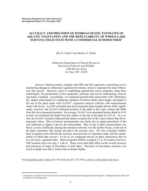
Fixed-point experiments–Divers located
and marked with numbered buoys, multiple
littoral zone microhabitats exhibiting a
variety of cover types, ranging from monotypic
stands of dense vegetation, to diverse
stands, to long, solitary coontail or whitestem
pondweed P. praelongus growing at the edge
of the littoral zone. At the surface, divers held
the transducer in place directly over the area
marked by the buoy and the area was pinged
numerous times until a consistent signal directly
over the targeted area was achieved.
After each of the buoy sites were pinged, divers
marked four corners of the ensonified
area with marker buoys. The four buoy strings
were held together at the surface by one diver,
thus creating a pyramid-shaped sampling area,
approximately equal to the size and shape of
the acoustic cone. The second diver descended
to the bottom, identified the tallest
plant intercepting the simulated cone, and
marked its length on a buoy string. Bottom
depth at the sediment-plant interface and plant
height were recorded at each sampling station
by a diver. Bottom depth and plant height
were also recorded with the echosounder and
EcoSAV. To account for the minor vagaries of
a stationary acoustic signal (i.e., ambient in
situ noise has a small effect the backscattering
of an acoustic signal), the mean depth and
plant height from a collection of 8 – 241 pings
at each fixed-point were calculated. Standard
deviations were calculated to determine the
quality (i.e., precision) of each acoustic estimates
at each fixed-point. One-sample t-tests
3

evaluating the null hypothesis that differences
between diver-measured and EcoSAVestimated
depths and plant heights were zero
(α = 0.05).
Whole-lake surveys–We completed
three mapping runs on consecutive days, targeting
the same GPS transects using a Garmin
® GPSmap 76 handheld GPS unit with
WAAS (Wide Area Augmentation System)
differential-correction enabled. We mapped
biovolume using methods described by Valley
et al. (2005). Briefly summarized, this entailed
collecting hydroacoustic vegetation data
over transects perpendicular to the longest
shoreline spaced 10 m apart. Boat speed was
2 – 4 knots, separating DGPS reports every 3
– 5 meters. This represented the distance
between data records and defined the size of
the ping cycles (typically 10-11 pings per
cycle). EcoSAV records one data location for
each record as the mid point between GPS
cycle boundaries. From the plant variables
reported by EcoSAV, we calculated percent
biovolume for each ping cycle using the following
formula:
Biovolume (%) =
⎛ PlantHeight
⎜
⎝ Depth
⎟
⎠
⎞
x Plant Cover
where: PlantHeight = the mean plant height
for only those pings signaling the presence of
plants; Depth = a best depth estimate for a
ping cycle determined from a patented heuristic
algorithm (Sabol and Johnston 2001); and
Plant Cover = the percent of all pings in a report
cycle signaling the presence of plants. To
estimate plant height, EcoSAV subtracts the
distance where the signal crosses the threshold
for plant detection from the distance to the
bottom signal (typically the sharpest rise in
voltage).
Biovolume at all unsampled areas was
estimated and mapped by kriging, which is a
geostatistical interpolator and smoother (Isaaks
and Srivastava 1989; Figure 1). We tested
the precision and accuracy of biovolume estimates
at the whole-lake scale by collecting
one independent set of verification data in
each lake along transects approximately perpendicular
to the map transects. For comparisons
to predicted values, we assumed
verification data sets were true measures.
4
Navigation error was computed in ArcView for
each survey as the root mean squared error
(RMSE) of the distance of the recorded track
points from the targeted transect line.
Exploratory data analysis from our
previous study and this one showed a negative
relationship between biovolume and depth.
Therefore, models relating biovolume to
depth and spatial location were constructed
from each whole-lake survey and then used to
predict biovolume across all grid cells of the
lake. Models were fitted in two steps. First, a
nonparametric regression smoother was fitted
with R to describe the relationship of biovolume
to depth and to remove this trend
(Chi-square p < 0.001). Next, the local spatial
patterns within the detrended residuals were
fitted by kriging. Finally, for each grid cell,
the predictions from the regression and kriging
were added to produce a predicted biovolume
accounting for both depth and local spatial
patterns (Valley et al. 2005). Biovolume grids
were imported into ArcView with Spatial Analyst
2.0 for all other GIS analyses.
We evaluated results from the wholelake
study at two levels of resolution: (1) consistency
of kriging predictions and model fits
to verification data over the entire littoral surface,
and (2) consistency of individual 5-m
grid cell predictions produced after repeated
surveys. Model fit was assessed by regressing
predicted grid cell biovolume values against
corresponding verification data recorded
within the same grid cell. All residuals from
these regressions were normally distributed
about the regression line. Adequacy of maps
for each lake was examined by qualitative
comparisons of mean squared errors (MSE),
and percent reductions in unexplained variance.
To evaluate whether predictions for the
whole-lake surveys were accurate, we compared
verification means to the mean predicted
values and the 95% confidence intervals
around the mean predicted biovolume. At the
local scale, the standard deviation of predictions
for individual grid cells over the three
days (n = 3) was calculated to describe the
precision of biovolume estimates. Because we
identified lower map precision at shallow littoral
depths (Valley et al. 2005), we evaluated
local survey precision in biovolume along a
gradient of littoral depth.

Square Lake
A
Vegetation
Biovolume
0%
100%
Figure 1. The abundance and distribution of submersed vegetation biovolume in Square
Lake. Map created by interpolating hydroacoustic measurements of vegetation
biovolume with kriging in GIS.
All map analyses were made for the
vegetated zone of each lake, which we define
as the littoral zone. The outer boundaries of
the littoral zone were defined by the average
maximum depth of contiguous bottom coverage
of vegetation, interpreted from a sample of
10 – 15 transects from each survey. Transects
were sampled uniformly across the littoral surface
of each lake. Sparse vegetation growing
at deeper depths was omitted from analysis.
Tests of location error–Estimates of
navigation error were a function of actual
driver error and location error from our DGPS
unit. To approximate location error, we conducted
seven fixed-transect experiments on
Square Lake over seven days in July 2004.
Transect lengths ranged from 50 to 100 m,
were arranged perpendicular to shore, and were
distributed evenly around the perimeter of
the lake. Transects were fixed with marker
buoys spaced 1 m apart. A swimmer equipped
with the DGPS completed three passes along
the length of the transect. Tracks (a collection
of points) from each pass and from each transect
were uploaded as themes into ArcView.
Because we could not identify the true location
of the fixed transects, a reference line was
placed parallel to each transect theme, and
distances of DGPS records from the line were
computed. The standard deviation of these
distances represented the average location error
for each transect. The mean standard deviation
from the seven transects represented
the average location error for the entire lake.
5

RESULTS
Fixed-point experiments−EcoSAVestimated
plant height did not significantly
differ from diver-measured plant height (one
sample t-test p=0.36). We did, however, find
appreciable differences between divermeasured
and EcoSAV estimated bottom depths
and top of plant depths. EcoSAV estimated
bottom depth was 0.18 m (+0.18 m SD)
deeper on average than diver-measured bottom
depth (one sample t-test p

20
A
Mean = -0.18
15
Count
10
5
0
-1.0 -0.5 0.0 0.5 1.0
Depth Error (m)
8
7
B
Mean = -0.23
6
5
Count
4
3
2
1
0
-1.0 -0.5 0.0 0.5 1.0
Top of Plant Error (m)
Figure 2. Histograms of the distribution of EcoSAV estimation errors (EcoSAV-estimate −
diver-estimate) from the fixed-point experiments. A) water depth errors (EcoSAVestimated
depth was deeper than diver measured depth). B) top of plant errors
(Top of plant signals were deeper than diver estimates). Means from both distributions
were significantly different from zero (one sample t-test p < 0.001).
7

EcoSAV ® -estimated Depth to Plant Tops (m)
-7
-6
-5
-4
-3
-2
-1
-0
I
F
N F I FN
R W I
R FW
S
F
C*
W
FN N
N
W
NF
M
N*
C
C*
C
F*
C*
C*
C
C
1:1 line
-0 -1 -2 -3 -4 -5 -6 -7
Diver-measured Depth to Plant Tops (m)
B
B
M
Figure 3. Depth to top of plant signal estimated with EcoSAV plotted against depth to top
of plant surveyed by divers over the ensonified area. Letters represent the species
of the tallest plant intercepting the cone [B = Bare, C = coontail, F = flatstem
pondweed P. zosteriformis, I = Illinois pondweed P. illinoensis, M = Chara spp.,
N = northern watermilfoil, R = Richardson’s pondweed P. richardsonii, S = sago
pondweed P. pectinatus, W = whitestem pondweed P. praelongus. Asterisks denote
where standard deviations of acoustic samples were greater than 0.1 m indicating
imprecise acoustic estimates of height (see METHODS).
8

Table 1. Results from GPS location error transect experiments in Square Lake in 2004. PDOP = position dilution of
precision.
Date Transect PDOP
Standard Deviation
(from arbitrary line of reference)
July 20 1 2.44 0.61
July 21 2 2.41 1.22
July 22 3 2.40 1.38
July 26 4 1.80 1.56
July 27 5 1.62 1.19
July 29 6 2.12 0.99
July 30 7 1.19 0.67
Mean Standard Deviation of Repeated
Biovolume Estimates (% ± SD)
13
12
11
10
9
8
7
6
5
4
3
2
1
0
13
12
11
10
9
8
7
6
5
4
3
2
1
0
Square Lake
1 2 3 4 5 6 7 8
Christmas Lake
1 2 3 4 5 6
Depth Bin (m)
Figure 4. Survey precision as a function of depth. Standard deviations of repeated biovolume
estimates were calculated for each 5-m grid cell. The mean of these is
then the measure of survey precision (± associated standard deviation) (n = 3 for
1000’s of 5-m grid cells) in Square and Christmas lakes (± associated standard
deviation).
9

Table 2.
Percent vegetation biovolume mean squared error (MSE) from the depth smoother (smoothed with 8-10 df), kriging interpolation model, mean biovolume from
verification samples, mean biovolume estimated from kriging, and navigation root mean squared error (RMSE) for three repeated surveys in each study lake.
Lake
Day
Total
Biovolume
Variance
Depth
Smoother
MSE a
Kriging
MSE a
Percent Total
Explained
Variance
Mean
Verification
Biovolume
(± 95% CI)
Mean
Kriging
Biovolume
(± 95% CI)
Navigation
RMSE
(m)
Square 1 317.5 176.5 95.3 70 23.8 ± 0.7 24.9 ± 0.7 4.7
2 294.0 156.9 89.5 70 -- 24.8 ± 0.7 4.0
3 276.5 151.2 71.1 74 -- 23.7 ± 0.6 3.6
Christmas 1 350.4 292.0 248.2 29 40.1 ± 0.7 38.9 ± 0.4 3.5
2 423.0 350.2 273.2 35 -- 41.9 ± 0.5 3.7
3 458.8 364.6 291.7 36 -- 41.5 ± 0.5 3.9
a The units for squared errors are squared percentages
10

much smaller than our reported errors. However,
it is important to note that error estimations
from Sabol et al. (2002) represent
differences between average predicted and
average observed plant heights within ensonified
0.3m x 0.3m quadrats, and not over individual
plants like our fixed-point experiments.
Because Sabol et al. (2002) averaged data over
larger sampling units than our study, the central
limit theorem, in part, may explain their
smaller errors.
Whole-lake surveys–Our methods
produced consistently accurate and precise
maps of biovolume for Square Lake. For
Christmas Lake, maps were accurate but not
precise. These results for Christmas Lake are
contrary to results published by Valley et al.
(2005) that documented high map precision in
this lake. However, in our earlier study, we
extended analyses to a depth of 8 m in both
Square and Christmas lakes. This depth was
an appropriate cut-off for analyses in Square
Lake because vegetation usually covered all
bottom areas close to 8 m deep. However, in
Christmas Lake, vegetation was sparse beyond
6.2 m. Biovolume in areas between 6.2 m and
8 m in Christmas lake was often zero, thus
artificially inflating map precision. The effect
of analysis boundaries on statistical distributions
illustrates the importance of carefully
defining the boundaries of the littoral zone.
Morris (1992) defined the littoral zone as the
area of shallow fresh water in which light
penetrates to the bottom and nurtures rooted
plants. Our operational definition as a zone of
contiguous bottom cover by vegetation fits this
concept.
Valley et al. (2005) demonstrated that
the degree of agreement between verification
and predicted data increased as littoral depth
increased. Similarly, in this analysis, as depth
increased, our survey precision increased as
well. Lower survey and map precision at shallow
depths is not surprising given the suite of
localized disturbances that cause vegetation
patchiness in such areas (e.g., harvesting,
sedimentation, wind/ice scour). In addition,
small deviations in plant height in shallow
depths lead to large deviations in biovolume.
As a result, we suggest focusing greater sampling
effort at depths less than two meters and
less effort at deeper depths. Fortunately,
kriging is not greatly affected by unbalanced
survey designs, and its behavior as a smoother
makes it robust to modest environmental noise
(Isaaks and Srivastava 1989). Ultimately, the
scale of the question and level of spatial resolution
supported by the data must be carefully
considered prior to interpreting results.
REFERENCES
Burks, R. L., E. Jeppesen, and D. M. Lodge.
2001. Littoral zone structures as
Daphnia refugia against predators.
Limnolology and Oceongraphy
46:230-237.
Christensen, D. L., B. R. Herwig, D. E.
Shindler, S. R. Carpenter. 1996. Impacts
of lakeshore residential development
on coarse woody debris in
north temperate lakes. Ecological Applications
6:1143-1149.
Canfield, D. E., J. V. Shireman, D. E. Colle,
W. T. Haller, C. E. Watkins II, and M.
J. Maceina. 1984. Prediction of chlorophyll
a concentrations in Florida
lakes: importance of aquatic macrophytes.
Canadian Journal of Fisheries
and Aquatic Sciences 41:497-501.
Collins, W. T., R. S. Gregory, and J. T.
Anderson. 1996. A digital approach to
seabed classification. Sea Technology
37: 83-87.
Drake, M. T., and R. D. Valley. 2005. Validation
and application of a fish-based
index of biotic integrity for small central
Minnesota lakes. North American
Journal of Fisheries Management
25:1095-1111.
Duarte, C. M. 1987. 1987. Use of echosounder
tracings to estimate the
aboveground biomass of submerged
plants in lakes. Canadian Journal of
Fisheries and Aquatic Sciences
44:732-735.
Isaaks, E. H., and R. M. Srivastava. 1989. An
introduction to applied geostatistics,
Oxford University Press, New York.
Jennings, M. J., M. A. Bozek, G. R. Hatzenbeler,
E. E. Emmons, M. D. Staggs.
1999. Cumulative effects of incremental
shoreline habitat modification
11

on fish assemblages in north temperate
lakes. North American Journal of
Fisheries Management 19:18-27.
Maceina, M. J., and J. V. Shireman. 1980. The
use of a recording fathometer for determination
of distribution and biomass
of Hydrilla. Journal of Aquatic
Plant Management 18:34-39.
Morris, C. 1992. Academic press dictionary of
science and technology. Academic
Press, Inc. San Diego.
Pouliquen E., and X. Lurton. 1992. Sea-bed
identification using echo sounder signal,
European Conference on Underwater
Acoustics. Elsevier Applied
Science, London.
Radomski, P., and T. J. Goeman. 2001. Consequences
of human lakeshore development
on emergent and floating-leaf
vegetation abundance. North American
Journal of Fisheries Management
21:46-61.
Rossi, R. E., D. J. Mulla, A. G. Journel, and E.
H. Franz. 1992. Geostatistical tools
for modeling and interpreting ecological
spatial dependence. Ecological
Monographs 62:277-314.
Sabol, B. M., J. Burczynski, and J. Hoffman.
2002a. Advanced digital processing of
echo sounder signals for characterization
of very dense submersed aquatic
vegetation. U.S. Army Engineers Research
and Development Center,
Technical Report ERDC/EL TR-02-
30. Vicksburg.
Sabol, B. M., and S. A. Johnston. 2001. Innovative
techniques for improved hydroacoustic
bottom tracking in dense
aquatic vegetation. US Army Corps of
Engineers Research and Development
Center, Tech. Rep. ERDC/EL MP-01-
2. Vicksburg.
Sabol, B. M., and R. E. Melton, Jr. 1995. Development
of an automated system for
detection and mapping of submersed
aquatic vegetation with hydroacoustic
and global positioning system technologies.
Report 1: the submersed
aquatic vegetation early warning system
(SAVEWS)-System description
and user's guide (Version 1.0). Joint
Agency Guntersville Project Aquatic
Plant Management, Nashville.
Sabol, B. M., R. E. J. Melton, R. Chamberlain,
P. H. Doering, and K. Haunert.
2002b. Evaluation of a digital echosounder
system for detection of submersed
aquatic vegetation. Estuaries
25:133-141.
Schriver, P., J. Bøgestrand, E. Jeppesen, M.
Søndergaard, 1995. Impact of submerged
macrophytes on fish–
zooplankton–phytoplankton interactions:
large-scale enclosure experiments
in a shallow eutrophic lake.
Freshwater Biology 33:255-270.
Thomas, G. L., S. L. Thiesfeld, S. A. Bonar,
R. N. Crittenden, and G. B. Pauley.
1990. Estimation of submergent plant
bed biovolume using acoustic range
information. Canadian Journal of
Fisheries and Aquatic Sciences
47:805-812.
R Development Core Team, 2003. The R
reference manual. Network Theory
Limited, UK.
Valley, R. D., M. T. Drake, and C. S. Anderson.
2005. Evaluation of alternative
interpolation techniques for the mapping
of remotely-sensed submersed
vegetation abundance. Aquatic Botany
81:13-25.
Wiens, J. A. 2002. Riverine landscapes: taking
landscape ecology into the water.
Freshwater Biology 47: 501-515.
12