Operating Instructions Manual For The Acoustic ... - BioSonics, Inc

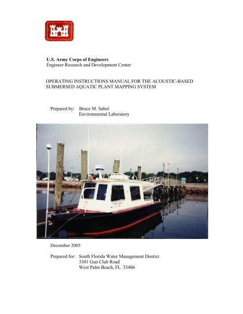
U.S. Army Corps of EngineersEngineer Research and Development CenterOPERATING INSTRUCTIONS MANUAL FOR THE ACOUSTIC-BASEDSUBMERSED AQUATIC PLANT MAPPING SYSTEMPrepared by: Bruce M. SabolEnvironmental LaboratoryDecember 2003Prepared for: South Florida Water Management District3301 Gun Club RoadWest Palm Beach, FL 33406

IntroductionThis brief instruction set is intended to serve as a guide for the use of the ERDC-developedSubmersed Aquatic Vegetation Early Warning System (SAVEWS) embodied in the BiosonicsDT-X sounder with a Leica MX-420 DGPS Navigation System and a Panosonic Toughbookcomputer. Instructions are written around the Biosonics Visual Acquisition software (version5.0.3), Biosonics EcoSAV software (version 1.0) which contains the windows SAVEWSsoftware, and the Leica MX-420 software (version 1.5). These instructions are not intended toreplace the separate instruction manuals for these components. Rather, the user is encouragedto study these separate manuals and to use this instruction set as a reminder during fieldoperations.Parts List• Biosonics DT-X Sounder (grey Pelican case with external connectors)• Biosonics DT-X transducer (420 kHz, 6-degree single beam)• Biosonics DT-X transducer cable• Biosonics GPS cable with mil-spec metal and DB-9 connectors• Biosonics power cables (AC and DC)• Biosonics ethernet cable (blue)• Panasonic Toughbook PC (with touch screen)• Panasonic AC power cable• Leica MX-420 DGPS• Leica DGPS Smart Antenna• Leica DGPS cable (3 signal connectors and 1 cigarette-lighter 12-volt plug)• Colored ribbon cable with DB9 connectors (only used for uploading and downloadingdata between GPS and PC)Connecting Equipment1. Connect DT-X transducer cable to the transducer. Verify that the rubber O-ring is inplace on the cable end (replacements are taped inside the sounder case). Hand-tightenthe plastic connector (NEVER user pliers to tighten or loosen).2. Connect other end of the transducer cable to TRANSDUCER 1 slot (TRANSDUCER 2slot is not active) on the back side of the DT-X sounder. The plug should be rotated sothat the grooves match, then pushed it in place while tightening the threaded ring tosecure the connection.3. Connect a DT-X sounder power cable using either the AC or the DC cable, but NOTboth. Power connectors on the back of the sounder are labeled and each has a uniquenumber of pins. Biosonics recommends using AC power, but in its absence DC works-2-

fine for a fully charged 12-volt battery (recommend monitoring battery voltage andswapping batteries when voltage drops below 12.3 volts).4. Connect Biosonics GPS cable to GPS slot on back of DT-X sounder.5. Connect blue ethernet cable to DT-X sounder (mil-spec connector on left out side ofsounder box) and to the PC (forward-most slot on right side of computer).6. Connect AC power supply cable to PC (slot on right rear side of PC).7. Connect 18-pin plastic connector on Leica GPS cable to the back of the MX-420 GPSdeck unit. Hand-tighten only.8. Connect the 10-pin plastic connector on GPS cable to Leica DGPS Smart Antenna.Hand-tighten only. Suggest taping the wire near the connector to the attached pipe tokeep tension off the plastic connector.9. Connect GPS cable power plug to 12-volt power supply with cigarette-lighter plug.10. Attach connectors on Leica cable and Biosonics GPS cable. Put electrical tape over theconnection to seal out water.11. Attach DT-X transducer to its mounting bracket and lower transducer into the water tosubmerse the entire transducer.12. DGPS antenna should be mounted with the white disk oriented horizontally with anunobscured view of the sky. It is desirable to place the antenna as close as possible todirectly above the transducer.Power Up Sequence1. GPS. Power up GPS by pressing the button on the lower right face of the GPS - buttonis marked with a while circle containing a while vertical line. A red light will appear onthe upper left face of the GPS. As satellites are acquired the light will change toorange. When the GPS is fully operational the color will change to green. It may takeup to 15 minutes to become fully operational.2. PC. Power up PC by depressing the silver knob on the right front of the PC. WindowsXP will be initiated.3. Sounder. Power up the sounder by toggling the black ON/OFF switch inside thesounder box on the right side. A red light will illuminate above the switch. Wait about30 seconds for a 3-beep tone to sound indicating that the sounder is operational.-3-

4. Visual Acquisition software. On the PC select (double click or touch the screen) theVisual Acquisition icon. Next, select “INIT DTX” (button on upper left of PC screen),a system information window will appear. This contains transducer information andrequires no input other than selecting “OK.” If you get the message “Could not identifytransducer,” recheck the transducer connections (steps 1 and 2 of ConnectingEquipment). Next, select “CONFIG DTX” - the Configure Echo Sounder window willappear. Specific input parameters are required in this window which are critical toplant detection operations. These are contained in a file which is called by clicking onLOAD. Select file SFWMD_01 (10 m depth limit) or SFWMD_02 (6 m depth limit)depending on maximum depth of area to be surveyed. Open this file then select OK. Ifother depths are required these may be manually typed into the configuration window.Parameter settings necessary for plant detection are listed below:WINDOW PARAMETER VALUE OR SETTINGReceiver Operating Mode Single BeamDataCollectionParametersEnvironmentalParametersData LoggingOptionsPulse ControlAcoustic ModeStart RangeEnd RangeThreshold LevelThreshold ModeTemperatureDepthpHSalinityAutomatic Data File CreationDatafile NamingPulse RatePulse DurationModeTransmit Power Reduction0 m (CRITICAL)slightly greater than maximum depth-130 dB (CRITICAL)squaredWater quality measurements needed tocompute speed of sound and adsorption.Set to midrange of values expected forsampling excursion. Use of exact valuesis not critical for shallow water SAVsurveys. Select COMPUTE, then OKBy Time, every 30 minutesTime Stamped (CRITICAL) , select OK10 pings/sec (suggested)0.1 ms (CRITICAL)Active Transmission (CRITICAL)0 dB5. Check GPS Signal. Latitude and longitude should be displayed in a widow on thelower right of the PC screen and the slash mark should be moving back and forth,indicating that an active stream of data is being read. If hash mark not moving, checkGPS connections and restart GPS.-4-

6. Activate Sounder. Select START PINGS button. The program will ask you to verifythat transducer is in water. After checking select YES. An echo intensity graphic willappear on the left side of the screen and an oscilloscope graphic will appear on the rightside. The system is now fully operational and ready for use. While transiting to thesurvey site it maybe desirable to take transducer out of the water. Before doing so,select PAUSE PINGS.Data Collection Operations1. Positioning Transducer. Place transducer in water fully submersing it. Depth shoulddepend on water roughness and the shallowest depth you plan to survey. Measure thedistance between the transducer face (bottom) and the water’s surface and record it inthe field book for later use by the tide-correction post-processing program.2. Begin Pinging. Start pinging, either by selecting START PINGS or RESUME PINGS.3. Logging Data. Select LOG DATA when the GPS navigation indicates that the datastart waypoint has been reached. Record the filename (data/time in lower left windowof PC) and the associated reach and transect number. Files are named using a 15-character date/time convention, which is needed for the post-processing program.4. Closing Data File. When GPS navigation indicates the stop data waypoint has beenreached, select CLOSE LOG (but do not take transducer out of the water). Optionally,you may want to select PAUSE PINGS and remove the transducer from the water if thenext measurement station is far away.5. Collecting Tide Data. Always measure and record the local tide data immediatelybefore and after conducting a survey. Additionally, if the survey runs for more than 2hours, it is advisable to record a mid-point tide measurement. These measurements willbe used by the post-processing program to make depth corrections.6. Data Integrity Check. Before leaving an area, it is recommended that you quicklyverify that the DT4 files are present and of the right size. This can be examined usingWindows Explorer or, better yet, using the replay option within the Visual Acquisitionsoftware.Power Down Sequence1. PC. Select STOP PINGS.2. PC. Select “Setup” from top list in window, then select “Shutdown EmbeddedController” from the menu list. Wait for window to tell you it is ready to power downthe DT-X sounder unit. Select YES to acknowledge shutdown.-5-

3. DT-X Sounder. Turn off DT-X sounder power switch.4. PC. Select “Setup” from top list in window, then select “Exit Visual Acquisition.”5. GPS. Turn off GPS.EcoSAV ProcessingThe EcoSAV software processes the raw binary acoustic file (DT4) to ASCII files (ODF)containing a series of position-referenced attributes, including depth, plant coverage, and plantheight. Parameters used in this processing are specified by an INI file which is tailored for theparticular environment sampled. Since SAVEWS was developed and refined on theCaloosahatchee, these parameters are well known for this site and are contained in the fileSFWMD_nn.INI (Figure 1). Even so, it will be necessary to adjust a few parameters from timeto time, and for different locations within the Caloosahatchee. Adjustments to the INI file maybe made outside of EcoSAV using any text editor, or interactively within the EcoSAVprogram. A full discussion of these parameters may be found in the Biosonics EcoSAV User’sGuide.1. Select Files to Process. Select the EcoSAV icon on the PC screen. The BioPlantwindow appears. Select File/Open. Acoustic survey data are stored in theC:\Biosonics\DTx\Data directory (default) as DT4 files. Select single or multiple files(control/click) and select OPEN. These files appear in the INPUT QUEUE window.2. Select Processing Parameter File. A generic INI file, suitable for the Caloosahatchee(SFWMD_01.INI), has been set as the system default, so generally it will not benecessary to change processing INI files and the user can proceed directly to step 3,below. However, occasionally changes will be necessary. Following instructions arefor substitution of an alternate INI file. Double click on first file in the queue window.The JOB PARAMETERS window appears select the Job Parameters tab. Within INISOURCE select SPECIFY AN INI and select BROWSE. Select SFWMD_nn (or otherpre-edited INI file) and select OPEN. Within OUTPUT FILE select “Append outputextension to the source filename.” Within OUTPUT NAMING RULES select“Overwrite output filename if it exists.” Select OK.3. Initiate Processing. At the bottom of the BioPlant Window select STARTPROCESSING FILE. The selected filename will appear in the Processing Queuewindow to indicate that processing is underway. When complete, the same filenamewith an ODF extension will appear in the Output Queue.4. Viewing Output. Double click on the ODF file in the Output Queue and the contentswill be displayed in the OUTPUT REPORT window (Figure 2). The upper portion ofthis window shows the Configuration Data used in the selected INI file. This isimportant because output results may change considerably by changing the parametervalues within the INI file. Actual output is shown below the configuration data.-6-

Position and time/date variables are derived from the GPS and represent whatevercoordinate system and time zone specified within the GPS. All remaining variables arederived from the processing of the acoustic data. Time and date will be needed in postprocessing to correct for tide. The BOTTOM depth is the distance between thetransducer face (bottom of transducer) and the detected bottom. Post-processingcorrections are required to account for the depth of the transducer and tides. A fulldiscussion of the output variables may be found in the Biosonics EcoSAV User’sGuide.5. Editing Processing Parameter File. It will be necessary from time to time to makechanges to the processing parameters in the INI file. The most likely parameter tochange would be the MAXIMUM PLANT DEPTH. This serves to prevent thealgorithm from looking for plants at depths exceeding the maximum depth of plantcolonization, which serves to minimize false alarms. For the Caloosahatchee a valuearound 2.3 m is about right under all conditions except exceedingly high tides. Thisand other parameters can be changed using an editor outside of the EcoSAVenvironment. Another approach is to make the change interactively within EcoSAV.To do this, select SETTINGS then EDIT AN INI FILE. Select and open the INI file toedit. Four tab windows will appear (Figure 3). The SITE SPECIFIC folder controlsoutput suppression and maximum plant depth limits (most likely screen to needchanging). No changes would likely need to be made to the SYSTEM SPECIFICscreen unless a different transducer was used. Conditions may arise requiring somechanges to ADVANCED and ADDITIONAL PARAMETERS screens, but it is notrecommended to change these without consulting Biosonics or Bruce Sabol. After allchanges have been made select SAVE and proceed with processing as described above.-7-

Figure 1. Default setting of SFWMD_01.INI optimized for Caloosahatchee estuary.[System Related Parameters]Signature = Aquatic Plant SoftwareVersion = 2Output Control = Rename[Site Specific Parameters]Gps Qualifier = 1Noisy Pings = 3Out of Water = 2Maximum Plant Depth = 2.200000[System Specific Parameters]Layer Height = 0.018000Calibration Correction = 0.000000Attenuation = 0.000000Near Field = 0.200000[Advanced Parameters]Threshold for Noise Checking and Plant Detection = -65Noise Checking Distance = 10Plant Detection Distance = 5Plant Height Threshold = 4Bottom Thickness Threshold = 12[Additional Parameters]Maximum Bottom Change = 0.110000B1 = -50B2 = 6B3 = 5B4 = 6P2 = -50P3 = 5P4 = -60P5 = 2P6 = -60Q1 = -125Q2 = 2R1 = 8-8-

Figure 2. Output report window.-9-

Figure 3. Editing an INI within EcoSAV.-10-

Post ProcessingThe post-processing program FINALIZE makes depth corrections, based on tide and transducerdepth, and concatenates individual ODF files into a single, space-delimited, ASCII text fileformatted in accordance with the metadata for the Caloosahatchee Estuary project. In additionto the ODF files to be included, the program requires a data file of tide measurements and a fileof ODF filenames with their associated reach, transect number, transducer depth and replicatenumber. Steps in creating these files and running FINALIZE are described below.1. Tide data file. An example tide file is contained in Figure 4. This ASCII spacedelimited text file can be generated using any text-editing program, such as MicrosoftWordpad or Notepad. The first line is for documentation only. Each subsequent linecontains the reach number, integer month, integer day of month, time (decimal hourslocal time), and tide (feet) relative to the selected reference plane. For each reach, thefirst line entry must contain a tide measurement BEFORE the first recorded ODF file.The last line entry for a given reach must contain a tide measurement AFTER the lastrecorded ODF file at that reach. If this condition is not met, the program will give awarning message and halt execution. If a tide measurement was not made at the correcttime during data collection, it will be necessary to estimate one and enter it. If the timespent at a reach exceeds 2 hours, it is recommended (but not imperative) that a mid-timetide measurement be added to the file.Figure 4.Tide data file must contain reach number, month, day, decimal hourlocal time, and tide (feet, NGVD29).{tide data SFW_21 6-9 Oct 2003: reach, mm, dd, hh.hh, tide}4 10 6 11.15 1.854 10 6 13.50 1.853 10 6 14.33 1.753 10 6 15.90 1.501 10 6 16.75 1.551 10 6 17.60 1.458 10 7 10.00 1.908 10 7 12.10 2.257 10 7 14.33 1.852 10 7 16.00 2.052 10 7 17.80 1.706 10 8 9.15 1.256 10 8 10.25 1.755 10 9 11.33 1.755 10 9 13.25 2.055 10 9 14.25 2.00-11-

2. File listing ODF files. An example file is contained in Figure 5. Each line of the filecorresponds to a single ODF file and its associated reach, transect number, depth of thetransducer face (meters), and replicate number. It is not critical to have this list orderedin any particular way, but it is convenient and customary to order the list by reach thentransect number - making it easier to find data from a given reach and transect in theoutput file. The easiest was to generate this file without having to type all the 15-character filenames is to enter the COMMAND PROMPT program (DOS emulator)and type: dir *.ODF > filelist.txt from within the proper directory. This will make a listof the ODF files in the current directory. Any text editor can then be used to discardeverything but the 15-character filenames. These should then be put in the proper orderwith a reach and transect number. Be careful to eliminate any aborted files from thelist.Figure 5.The list file must contain ODF filename, reach number, transect number,transducer depth (m) and replicate number.20031006_165545 1 1 0.25 120031006_170321 1 2 0.25 120031006_170916 1 3 0.25 120031006_171231 1 3 0.25 220031006_171559 1 4 0.25 120031006_172327 1 5 0.25 120031006_173050 1 6 0.25 120031007_165843 2 1 0.25 120031007_170446 2 2 0.25 120031007_171143 2 3 0.25 120031007_171909 2 4 0.25 120031007_172711 2 5 0.25 120031007_173510 2 6 0.25 120031007_174258 2 7 0.25 120031007_162633 2 8 0.25 120031007_163354 2 9 0.25 120031007_164054 2 10 0.25 120031006_143924 3 1 0.30 120031006_144934 3 2 0.30 120031006_145555 3 3 0.30 120031006_150130 3 4 0.30 120031006 150739 3 5 0.30 13. Running FINALIZE. Double click on the FINALIZE icon. The program will query theuser for the integer survey number (reference Caloosahatchee metadata documentation).The FORM1 window then appears; click Create Output File of Corrected Data.Specify the desired filename and directory location of the output file, then click Open.Select the filename and location of the file containing the list of ODF files; click Open.Select the filename and location of the tide measurement data, then click Open.-12-

Numbers in the FORM1 window will scroll by as the program executes. A successfulcompletion message window will appear when the program is done; click OK. Finally,close the FORM1 window to exit the program.4. Output file format. The format of the output ASCII space delimited .DAT file is inaccordance with the current metadata standard for the Caloosahatchee estuary project.Note that the metadata standard changed after survey 19 (March 2003) to include depthcorrected to the National Geodetic Vertical Datum (NGVD) 1929 reference plane. Anexample output .DAT file is illustrated in Figure 6.Figure 6. Output file.82.12839 26.50698 2002 206 14.8694 17 7 5 1 -1.88 40.00 0.3582.12840 26.50695 2002 206 14.8700 17 7 5 1 -1.88 45.45 0.4082.12840 26.50692 2002 206 14.8706 17 7 5 1 -1.85 40.00 0.3582.12840 26.50690 2002 206 14.8711 17 7 5 1 -1.81 27.27 0.2782.12842 26.50687 2002 206 14.8717 17 7 5 1 -1.81 50.00 0.2682.12843 26.50683 2002 206 14.8725 17 7 5 1 -1.81 43.75 0.1982.12843 26.50679 2002 206 14.8733 17 7 5 1 -1.81 20.00 0.1682.12844 26.50677 2002 206 14.8739 17 7 5 1 -1.76 45.45 0.3182.12845 26.50674 2002 206 14.8744 17 7 5 1 -1.74 30.00 0.2982.12845 26.50672 2002 206 14.8750 17 7 5 1 -1.72 90.00 0.4582.12845 26.50669 2002 206 14.8756 17 7 5 1 -1.67 81.82 0.4982.12845 26.50666 2002 206 14.8761 17 7 5 1 -1.63 80.00 0.4482.12845 26.50664 2002 206 14.8767 17 7 5 1 -1.59 90.91 0.4282.12845 26.50661 2002 206 14.8772 17 7 5 1 -1.52 80.00 0.36As per the metadata description, each record contains the following variables:longitude - decimal degrees W longitude in NAD83latitude - decimal degrees N latitude in NAD83year - four digit yearday - Julian daytime - decimal hours Greenwich Mean Timesurvey - sequential survey numberreach - reach number (1-8)transect - transect numberreplicate - replicate numberdepth - depth of detected bottom in meters relative to NGVD29coverage - estimated plant coverage in percentheight - mean plant height (m)5. Documentation on FINALIZE. Finalize is written in Visual Basic 6.0 and should workwell with any PC running Windows XP. The installation CD (attached to this report)contains the source code (directory FINALIZE_source) and installation software-13-

(directory FINALIZE). The source code will allow the user to modify the program asnecessary. Julian day is computed based on month, day, and year, and takes leap yearinto account. Tide corrections are determined by time-based linear interpolation usingthe date/time within the ODF filename; that is, all depths within a single transect aretide corrected by a single value.6. Installing FINALIZE. Insert the installation CD and open the FINALIZE directory.Click on SETUP.EXE and follow the installation instructions. It may be convenient togenerate a shortcut icon to activate the program. Click Start\Programs then right clickFINALIZE. Select Create Shortcut. Next, select the created shortcut file and drag anddrop it on the PC screen.GPS SetupThe MX-420 GPS has been initially configured for work properly with the DT-X sounder forplant mapping operations. Information below is provided to enable the user to reset theseconfiguration parameters should they get changed or be erased. All parameter setting isperformed using the configuration screens activated by pressing the CFG key on the lower rightof the GPS panel. This activates a split window with items listed on the left and correspondingconfiguration values on the right. Press the CFG key and scroll (large button with 4 arrows) toa specific item. To make a change to a configuration value press the E key (editor), make theappropriate change, then press the E key again to exit. The following settings are required foroperation with SAVEWS.DATUM/Datum = WGS-84NAVIGATION/WPT Pass Distance = 0.02kmNMEA OUT 1/Not ActiveNMEA OUT2/Port Active (yes), set GGA, GLL, ZDA output sentences to ON,all others OFFPOSITION/Reference System = Lat/LonPOSITION/Alarm if no update –> YESSERIAL I/O/4800 Baud for allTIME/Time System = UTCWPT&RTE In/External WPT Inputs –> YESNavigating with GPSThe Leica MX-420 GPS may be used to navigate a stored route (sequence of waypoints). Thisinvolves selecting the route (each sampling reach has a route with the same identificationnumber) then navigating the route. Select a route using the following sequence of commandson the GPS.1. Push the RTE button to display the RTE1 window.-14-

2. Enter the edit mode by pressing the E button.3. Press INSERT softkey (far left).4. Press INSERT ROUTE softkey (far right).5. Select the desired route number by scrolling down the list of routes with the cursorbutton.6. Press INSERT FORWARD softkey.7. Exit the edit mode by pressing the E key.Navigation may be performed using either the NAV or PLOT windows. The NAV3 window(press NAV button 3 times) provides a runway display with cross-track error bar. The PLOT1window (press PLOT button once) provides a plan view of the route and boat path. If itbecomes necessary to repeat a transect, repeat the route selection procedure described above.Enter the NAV3 window and enter the edit mode (E key). Repeatedly press the SKIPWAYPOINT softkey until the desired waypoint appears in the NEXT POINT box on theNAV3 window.Manipulating GPS WaypointsWaypoints may be moved between the GPS and the PC. Waypoints and routes used in theCaloosahatchee Estuary study have been loaded onto the GPS. Waypoints are stored on the PCin C:\Leica_GPS\WayPts01.txt. These data are in NMEA 0183 Standard Waypoint Locationformat (WLP) described on pp. 60-61 of the GPS operator’s manual. Uploading ordownloading waypoints requires altering the cable connections, temporarily reconfiguring theGPS, and running the WayPtIO program, stored in C:\Leica_GPS.1. Connections. Undo the connection between the GPS and the DT-X sounder. Connectthe GPS cable to the colored ribbon cable and connect the other end of the ribbon cableto the COM1 port on the back of the PC (only place it will connect).2. GPS Reconfiguration. Reconfiguration steps (p. 62 GPS Operator’s Manual) includethe following:CFG\NMEA Out2, enter edit mode (press E key)Turn OFF all output sentencesTurn ON WPL output sentenceSelect “Details” using the softkey, set Checksum Yes for downloadset Checksum No for inital uploadset Include Waypoint name to YES,-15-

set Decimals to 4press Done softkeyTurn OFF WPL output sentenceThe port remains active (PORT ACTIVE= yes)3. Downloading Data (GPS to PC). Run the executable program WayPtIO stored on thePC in C:\Leica_GPS. Select Setup/COM Port - set Serial Port to COM1, and Baud to4800, select OK. Select Setup/Operational Settings - set the following:Output Interval =1Sentences per Interval = 1Checked boxes: Echo Transmit Data, Repeat Transmit Data, DisplayReceived Data, Save Received DataSelect Save Receive Data File and designate a location and filename forthe downloaded data.Select OK“Push” the green button on the PC program screen, then push the SEND ALL sortkey(on GPS), then “push” the red button on the PC program screen. Exit the program andverify that the file has been received.4. Uploading Data (PC to GPS). Run the executable program WayPtIO stored on the PCin C:\Leica_GPS. Select Setup/COM Port - set Serial Port to COM1, and Baud to 4800,select OK. Select Setup/Operational Settings - set the following:Output Interval =1Sentences per Interval = 1Checked boxes: Transmit, Echo Transmit Data, Display Received DataSelect Select File, and designate location and filename of uploaded data.Select OK“Push” the green button on the PC program screen. After the transmitted data hasstopped scrolling across the PC screen, exit the program and verify that the waypointlist (WPT key) on the GPS is correct. If correct, lock them in place by entering theeditor within the Waypoint window (press the E key). Press the More softkey on theGPS until the Lock all WPT softkey appears, press it, then exit the editor (press E key).5. Restore GPS Configuration. Remember to restore the NMEA Out 2 configuration asdescribed in GPS Setup, above (NMEA OUT2/Port Active (yes), set GGA, GLL, ZDAoutput sentences to ON, all others OFF).Entering GPS RoutesRoutes may likewise be entered via the PC using the NMEA Standard Rnn and RTE formats ina procedure similar to that described above. However, because of the limited number of routesused in the Caloosahatchee study, we have opted to enter them manually on the GPS using theprocedure described on p. 34 of the GPS operator’s manual. Steps required to enter multiplewaypointroutes are summarized below.-16-

1. Press the RTE key twice to get to the RTE 2 window which displays route banks.Scroll down to the route number to be populated or changed.2. Enter edit mode by pressing the E key. To populate a new route with previouslyentered waypoints press the Insert by numb. softkey.3. Enter the first waypoint number then press the Insert this WPT softkey. Repeat thisprocedure for each waypoint in the route.4. After the final waypoint has been entered (followed by pressing the Insert this WPTsoftkey) exit the edit mode by pressing the E key. Next, press the E key again. Inspectthe waypoints just entered. If they are correct press the Lock Route softkey. Routeentry is now complete.Suggestions1. Daily data archiving, write .DT4 files to an archival medium such as a CD, using theCD writer on the Toughbook PC.2. Periodically remove RTP, NME, and DT4 files from the data directory, after havingarchived them.3. Daily processing and quick graphic display of collected data, suggest using Surfer orother low end PC mapping software.4. Care and maintenance of equipment. All connectors are very fragile. A brokenconnector can cost a day’s work. Suggest taking extreme care of cables and connectors,including getting a toolbox with spare parts and tools to repair connectors and damagescables. This should include pin-out diagrams for all equipment. Damage to thetransducer cable requires a factory repair because it must be recalibrated.Point of ContactPlease provide comments or corrections to:Mr. Bruce Sabol, ATTN: CEERD-EE-CU.S. Army Engineer Research and Development Center3909 Halls Ferry Rd.Vicksburg, MS 39180-6199601-634-2297Bruce.M.Sabol@erdc.usace.army.mil-17-