MULTIBODY DYNAMICS 2007, ECCOMAS Thematic ... - BBAA VI

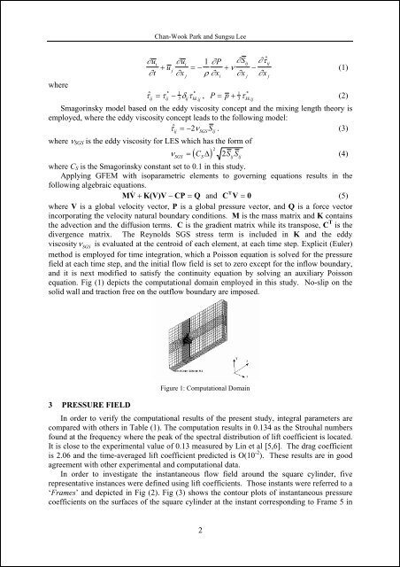
Chan-Wook Park and Sungsu Lee∂ui∂t∂u∂Pν ∂ S ∂τi 1 $ij ij+ uj= − + −∂xρ ∂x∂x∂xjwhere* *$ τij = τij − 1 3 δijτkk , P = p+ 1 ij3 τ * kk(2)ijSmagorinsky model based on the eddy viscosity concept and the mixing length theory isemployed, where the eddy viscosity concept leads to the following model:$ τ =−2 ν S . (3)ij SGS ijwhere ν SGS is the eddy viscosity for LES which has the form of( C )ν SGS SS ij ijijj(1)= Δ 2 2 S (4)where C S is the Smagorinsky constant set to 0.1 in this study.Applying GFEM with isoparametric elements to governing equations results in thefollowing algebraic equations.MV& + K(V)V − CP = Q and CT V = 0(5)where V is a global velocity vector, P is a global pressure vector, and Q is a force vectorincorporating the velocity natural boundary conditions. M is the mass matrix and K containsthe advection and the diffusion terms. C is the gradient matrix while its transpose, C T is thedivergence matrix. The Reynolds SGS stress term is included in K and the eddyviscosityν SGSis evaluated at the centroid of each element, at each time step. Explicit (Euler)method is employed for time integration, which a Poisson equation is solved for the pressurefield at each time step, and the initial flow field is set to zero except for the inflow boundary,and it is next modified to satisfy the continuity equation by solving an auxiliary Poissonequation. Fig (1) depicts the computational domain employed in this study. No-slip on thesolid wall and traction free on the outflow boundary are imposed.3 PRESSURE FIELDFigure 1: Computational DomainIn order to verify the computational results of the present study, integral parameters arecompared with others in Table (1). The computation results in 0.134 as the Strouhal numbersfound at the frequency where the peak of the spectral distribution of lift coefficient is located.It is close to the experimental value of 0.13 measured by Lin et al [5,6]. The drag coefficientis 2.06 and the time-averaged lift coefficient predicted is O(10 -2 ). These results are in goodagreement with other experimental and computational data.In order to investigate the instantaneous flow field around the square cylinder, fiverepresentative instances were defined using lift coefficients. Those instants were referred to a‘Frames’ and depicted in Fig (2). Fig (3) shows the contour plots of instantaneous pressurecoefficients on the surfaces of the square cylinder at the instant corresponding to Frame 5 in2