Summary 2. The electromechanical energy conversion

Summary
2. THE ELECTROMECHANICAL ENERGY CONVERSION .............................................................. 1
2.1 THE PRIMITIVE MACHINE ............................................................................................................ 1
2.1.1 The torque/speed curve ........................................................................................................... 2
2.1.2 Reluctance torque and excitation torque ................................................................................ 3
2.1.3 Motor nameplate and rated values ......................................................................................... 5
2. The electromechanical energy conversion
2.1 The primitive machine
Before addressing the study of electrical machines is convenient to introduce the study of the
basic principles of electromechanical energy conversion.
The starting point for understanding this theory is the primitive machine:
I
+ +
l
E
v
+
B
+
V
+ +
F
+ +
M,R
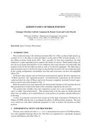
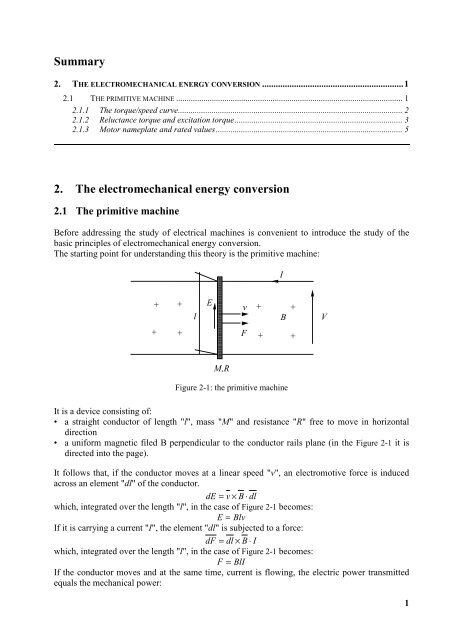
Figure 2-1: the primitive machine
It is a device consisting of:
• a straight conductor of length "l", mass "M" and resistance "R" free to move in horizontal
direction
• a uniform magnetic filed B perpendicular to the conductor rails plane (in the Figure 2-1 it is
directed into the page).
It follows that, if the conductor moves at a linear speed "v", an electromotive force is induced
across an element "dl" of the conductor.
dE = v × B ⋅ dl
which, integrated over the length "l", in the case of Figure 2-1 becomes:
E = Blv
If it is carrying a current "I", the element "dl" is subjected to a force:
dF = dl × B ⋅ I
which, integrated over the length "l", in the case of Figure 2-1 becomes:
F = BlI
If the conductor moves and at the same time, current is flowing, the electric power transmitted
equals the mechanical power:
1

F
P
e
= E ⋅ I = B ⋅l
⋅ v ⋅ = F ⋅ v = P m
B ⋅l
Consider, then, the evolution of the following phenomenon (the conductor is free to move):
• initial status: conductor is stopped and no current is flowing
• a voltage V is applied, so an initial current begins to flow: I o
= V / R
• it generates an electromagnetic force on the conductor: Fe
= B ⋅ l ⋅ I
o
• the conductor accelerates, and this generates an induced electromotive force: E = Blv
V − E
• in every instants you have, then, that the current becomes: I =
R
• equilibrium is reached when the current vanishes and therefore when V = E
If braking forces go into action, then the balance is reached when F
e
= Fr
and therefore the
presence of a current is required. In particular:
2 2
V − E Blvo
− Blv B l
Fr
= BlI = Bl = Bl = ⋅ ( vo
− v)
R R R
Fr
v = vo
−
2 2
B l
R
where "v" is always less than the no load speed v o .
What was said for for the primitive linear machine remains valid for a rotating machine, making
the appropriate substitutions:
• instead of the Bl product, the flux Ψ has to be considered
• the electromagnetic force F e becomes electromagnetic torque T e
• the linear speed v becomes angular speed Ω
• the inertia force becomes inertia torque
• the braking force becomes braking torque.
The fundamental relationships then become:
E = ΩΨ Te
= ΨI
EI = TeΩ
We can thus obtain, in a similar way, the values of the operating speed:
• at no load (without braking torque)
V
Ωo
=
Ψ
• at a load (with braking torque)
2.1.1 The torque/speed curve
Ω = Ω
−
T r
o 2
Ψ
The locus of the operation points (at steady state) of the electric machine is called torque/speed
curve. The remarkable points are:
• the intersection with the torque axis (zero speed = standstill), which represents the start
torque.
• the intersection with the speed axis (zero torque = no load), which provides no load speed.
The intersection of this curve with the torque/speed curve of the mechanical load identifies the
operating point.
This operating point can be stable or unstable.
R
2

Will be stable if an increase of speed is a deficiency of torque so the machine slows down;
conversely, a decrease of speed must be matched by a surplus of torque so the machine
accelerates.
Knowledge of the mechanical behavior of the load is a fundamental starting point for the drive
design and for the choice of the machine to be used.
By studying the behavior of the mechanical load, you can in fact identify the needs in terms of
torque, starting from the time profile of the required speed. You may also obtain the points of
maximum acceleration and deceleration, that are the points of maximum torque for the electric
machine.
2.1.2 Reluctance torque and excitation torque
In this section we want to highlight the different contributions to the birth of electro-mechanical
action.
Basically there are two different cases:
• torque resulting from the magnetic structure of the circuit, that is caused by anisotropy
• resulting from the interaction between two magnetic coils.
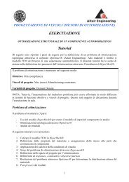
Consider the first case, referring to Figure 2-2, where you can highlight a magnetic structure
made by a fixed part on which is mounted a winding and a rotating part.
θ
v
i
Figure 2-2: reluctance torque in a primitive machine
From an electrical point of view, the system can be represented by a one-port as a series of a
variable resistor with an inductance. Thus we have:
d
di dL
v = Ri + ( Li)
= Ri + L + i
dt
dt dt
Multiplying both sides by he current "i", we obtain the equation expressing the energy balance:
2 di 2 dL
vi = Ri + iL + i
dt dt
Recalling that the instantaneous power absorbed by the magnetic field can be obtained by
differentiating the energy expression, it results:
dW d ⎛ 1 2 ⎞ di 1 2 dL
pµ
= = ⎜ Li ⎟ = Li + i
dt dt ⎝ 2 ⎠ dt 2 dt
3

Comparing this expression with the energy balance of the circuit, we find that the total electric
power inlet (on the left of the equation) is divided into three contributions:
• power dissipated in the resistance
2
p p
= Ri
• power related to the magnetic field
• mechanical power
p
µ
di 1 2
= Li + i
dt 2
1 2 dL
p m
= i
2 dt
If we consider that the inductance in the reference frame varies with periodic sinusoidal pattern,
you can highlight an expression for the anisotropy torque:
1 2 dL 1 2 dL dθ
1 2 dL
p m
= i = i = i Ω
2 dt 2 dθ
dt 2 dθ
pm
1 2 dL
Tm
= = i
Ω 2 dθ
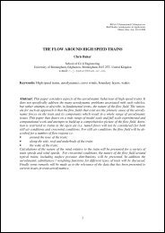
Now, suppose you change the old structure so as to also include a winding on the rotating part as
in Figure 2-3.
dL
dt
θ
i 2
v 2
v 1
i 1
Figure 2-3: reluctance and excitation torque in a primitive machine
The equations describing this structure are that of a mutual inductor with variable parameters.
You can then write:
d d
v1
= R1i1
+ ( L1i1
) + ( Lmi2
)
dt dt
d d
v2
= R2i2
+ ( L2i2
) + ( Lmi1
)
dt dt
and developing the derivatives:
di1
dL1
di2
dLm
v1
= R1i1
+ L1
+ i1
+ Lm
+ i2
dt dt dt dt
di2
dL2
di1
dLm
v2
= R2i2
+ L2
+ i2
+ Lm
+ i1
dt dt dt dt
4

If, therefore, similar to what we saw before, we extract the contributions related to the
mechanical power, it is obtained:
1 2 dL1
1 dLm
for the primary windings i1
+ i1i2
2 dt 2 dt
1 2 dL2
1 dLm
for the secondary windings i2
+ i1i2
2 dt 2 dt
In a similar way as before, we can highlight the following contributions to the torque:
1 2 dL1
1 2 dL2
dLm
Tm = i1
+ i2
+ i1i2
2 dθ 2 dθ dθ
where the first two terms are similar to the previous terms of anisotropy and the last torque is
called excitation torque:
dLm
Tm = i1i2
dθ
2.1.3 Motor nameplate and rated values
In order to be able to identify the characteristics of a machine is necessary to see the nameplate
that is located on the frame. This nameplate is a real ID card that allows us to trace the basic
features of the machine with regard to the application point of view. The values reported on the
plate depend on the type of machine, but they are able to provide the information for a proper
connection and use.
As we shall see later, however, the data are not useful for determining the appropriate design of
the control, given that certain parameters must be obtained experimentally and are rarely
supplied by the manufacturer.
The basic parameters set are called rated data and identify an operation point of the machine, at
which the engine can work indefinitely in time without thermal problems (apart from obviously
the wear).
2.1.3.1 Nomenclature notes for rotating machinery
• stator
• rotor
• inductor winding
• induced winding
part of the machine which remains stationary during operation
part of the machine which is in rotary motion during operation
winding that creates the main magnetic field
winding immersed in the field created by the inductor
5